WO2005045391A2

WO2005045391A2 - System and process for detecting substances

Info

Publication number: WO2005045391A2
Application number: PCT/AU2004/001542
Authority: WO
Inventors: Russell Wilkie
Original assignee: Elan Group Ltd
Priority date: 2003-11-06
Filing date: 2004-11-08
Publication date: 2005-05-19

Abstract

A system of calibrating spectra data for detecting substances including means for non-invasively acquiring a plurality of reflected spectra from each sample of a known substance; analysing means arranged to provide an averaged spectra data of the plurality of reflected spectra for each sample, and having one or more calibration models for analysing the spectra data to provide a comparison data, wherein the comparison data from the spectra data of the samples of known substances are for use as corresponding validation data sets, each set relating to the reflected spectra from the known substances of a specie; and storage means for storing the validation data sets.

Description

SYSTEM AND PROCESS FOR DETECTING SUBSTANCES

TECHNICAL FIELD OF THE INVENTION THIS INVENTION relates to a system/process for detecting substances, and

in particular but not limited to a system/process for detecting aflatoxin in peanut

meals.

BACKGROUND OF THE INVENTION

Systems and processes for automated detection of substances are desired in

many government departments, industries and commercial organisations as they

would allow automation of certain tasks that are currently done manually. Many of

these substances are microorganisms which are difficult or impossible to see with

naked eye. For example, an automated detection system would facilitate the food

production industry to detect harmful substances in foods such as aflatoxin in

peanut meal, during production and thereby preventing supply of any contaminated

food to other traders and consumers. Such detection system can also be adapted to

detect certain harmful, contagious, toxic or illegal substances in surveillance of

postal articles at a mail sorting center, containers, bags and suitcases in an air port

or shipping terminal.

In particular, in situations where a dangerous, contagious or poisonous

substance may be present only in some of the containers, parcels or products, it

would be advantageous to be able to identify the contaminated items for removal

in order to prevent people from being harmed. The recent anthrax scare in the

United States postal system is one such situation. In view of the desires to automate identification of substances in

governments, and the industrial and commercial sectors, many attempts to achieve

same have been made. Amongst the prior art attempts, spectroscopy is favoured as

it can be used for a non-invasive detection. However, the prior art spectroscopic

systems and processes are not sufficiently reliable for practical usage.

Further, an item presented for determination of its constituents may have

varying particle sized constituents, and these varying sizes tend to affect reliability

of spectroscopic measurements of the item. Accordingly, the accuracy of predicting

the constituents in such an item is low. OBIECT OF THE INVENTION

It is an object of the present invention to provide a relatively robust

system/process for detecting substances.

Another object of the present invention is to provide an apparatus for use in

detecting substances. SUMMARY OF THE INVENTION

In one aspect therefore the present invention resides in a system of

calibrating spectra data for detecting substances- The system includes means for

non-invasively acquiring a plurality of reflected spectra from each sample of a

known substance; analysing means arranged to provide an averaged spectra data

of the plurality of reflected spectra for each sample, and having one or more

calibration models for analysing the spectra data to provide a comparison data,

wherein the comparison data from the spectra data of the samples of known

substances are for use as corresponding validation data sets, each set relating to the reflected spectra from the known substances of a specie; and storage means for

storing the validation data sets.

The system may further include processing means adapted to analyse the

acquired spectra from a substance for detection with the calibration model to

provide a comparison data and to compare the comparison data with the stored

validation data sets for finding a matched or closely matched validation data set for

detecting the substance.

In another aspect therefore the present invention resides in a process of

calibrating spectra data for detecting substances. The process includes the following

steps:

(1 ) non-invasively acquiring reflected spectra from a plurality of samples of a

known substance;

(2) averaging and validating acquired spectra from samples of the known

substance to provide an averaged spectra data;

(3) with a calibration model analysing the averaged spectra data to provide a

comparison data, wherein the comparison data provided from averaged spectra data

of known substances are for use as corresponding validation data sets, each set

relating to the reflected spectra from known substances of a specie; and

(4) storing the validation data sets in storage means. The process may further include the step of:

(5) analysing the acquired spectra from a substance for detection with the

calibration model to provide a comparison data; and (6) comparing the comparison data with the stored validation data sets for

finding a matched or closely matched validation data set for detecting the

substance.

The averaged spectra may be grouped so that each group has a number of

averaged spectra data corresponding to samples with a specific range of a

constituent measurements of the known substance. The specific range can be

determined so that each group has reasonable similar numbers of the samples.

The acquired spectra or the averaged spectra data may be filtered so that

data from samples that are outside a range of constituent measurements are

removed before calibration.

The spectra acquiring means may be a spectrometer and preferably a near

infrared (N I R) spectrometer. More preferably, the NIR spectrometer is that described

in the applicant's corresponding PCT International Patent Publication Numbered

WO 99/61898. The disclosure of WO 99/61898 is fully incorporated herein by

reference.

In a further aspect therefore the present invention resides in an apparatus of

acquiring spectra data for detecting substances. The apparatus includes means for

non-invasively acquiring reflected spectra from a substance; analysing means

having one or more calibration models for analysing acquired spectra to provide a

comparison data, wherein the comparison data provided from acquired spectra of

known substances are for use as corresponding validation data sets, each set

relating to the reflected spectra from known substances of a specie, and storage

means for storing the validation data sets. The spectra acquiring means has an interactance probe arranged for illuminating the substance and a rubber boot fitted

on the probe. The rubber boot has a free end on which the object is positioned .

Preferably, said substance is an microorganism in a food item. The

microorganism may be afatoxin. Said food item may be a peanut meal or other nut

meal.

In preference, the analysing means/step is adapted to analyse spectra within

a predetermined optimal bandwidth or multiple bandwidths for each specie of

substances.

The calibration model may be any of the known mυltivariate models

including partial least squares (PLS), principal component regression (PCR) and

principal component analysis (PCA).

Desirably, the calibration model is adapted to present the comparison data

as a number or numbers for indicating closeness of matching a specie of substances

and the processing means/step is adapted to indicate a match when the number or

numbers is within a predetermined range of values. In one form the number or

numbers represent Mahalanobis (M) distance.

BRIEF DESCRIPTION OR THE EMBODIMENTS In order that the present invention can be more readily understood and be

put into practical effect reference will now be made to the accompanying drawings

which illustrate embodiments of the present invention and wherein:-

Figure 1 is a flow diagram showing certain functional modules of an

embodiment of the system according to the present invention; Figure 2 is a flow diagram showing certain functional modules of another

embodiment of the system according to the present invention; Figure 3 shows a calibration graph;

Figure 4 is a table showing calibrations at steps of the system according to

the present invention;

Figure 5 is a table showing results of the classification steps shown in Figure

4.

Figure 6 is a drawing showing an embodiment of an apparatus for acquiring

spectra data from a sample according to the present invention; Figure 7 is a plan view of the spectra acquiring station of the apparatus

shown in Figure 6; and

Figure 8 is a cross-sectional view of the spectra acquiring station shown in

Figure 7.

DETAILED DESCRIPTION OF THE DRAWINGS Referring initially to Figure 1 , there is shown a system 10 for detecting

substances according to one embodiment of the present invention. The system 10

has a spectra data acquiring module 14 for acquiring raw spectra reflected from the

substances or samples 12, The raw data are then analysed and calibrated with a

computer or processing means 16 using one of the PCA, PCR and PLS multivariate

calibration models 18. The calibrated data are then validated with laboratory test

results 20 to eliminate any outliers and to save the accepted data as validation data

sets for species of substances in storage means 22. The system 10 can then be used

to predict unknown substances by calibrating unknown sample spectrum 24 and comparing the calibrated unknown sample spectrum with the stored data sets from

the storage 22. The comparison result is displayed as prediction parameter at the

display unit 26.

The calibration process is briefly described below. Calibration development

is a requirement when using spectroscopy to non-destructively predict parameters

in "unknown" samples. There are two calibration types: quantitative and

qualitative.

A quantitative calibration generally describes prediction results in numerical

format (eg. Total soluble solids or TSS, Acidity, Firmness) and is used widely

throughout industry. To enable successful quantitative calibration development,

linear or non-linear relationships between spectral data and corresponding

laboratory results describe trends unique to that particular material.

A qualitative calibration may describe results in an identification format, and

is only recently been accepted in industry. To enable successful qualitative

calibration development, spectral data sets are grouped according to variety/type

and run through a series of mathematical steps before available for use.

Quantitative Calibrations

There are many quantitative cal ibration types. Classic univariate quantitative

models such as Least Squares Regression, Classical Least Squares (CLS) and Inverse

Least Squares (ILS) utilise clearly defined relationships between independent data

(spectral absorbances) and dependent data (concentrations). They therefore require

pure samples, a detailed knowledge of constituents present within the studied material and corresponding spectral bands, and knowledge of the concentration of

every constituent present within the material.

Because near-infrared spectrometers are "omnianalysers", multivariate

models such as Partial Least Squares (PLS) Model, Principal Component Regression

(PCR) and Principal Component Analysis (PCA) have been employed, where a

range of spectral variability is expected and little is known about the constituents

present within the material. They allow for inclusion of more data, and due to the

averaging process provide more "stable" results.

In these quantitative methods, large variations in spectral data should relate

somewhatto combined differences of all constituent concentrations present within

the material. Eigenvectors (spectral loadings or principal components) are used to

represent, in decreasing order of magnitude, the largest variations to the smallest

variations present within a set of spectral data. These relate to the constituent

concentrations in the original samples, and can predict unknowns; "the only

difference between spectra of samples with different constituent concentrations is

the fraction of each loading added (scores)".

Quantitative Calibration Steps and Algorithms: PCA/PCR

This is the most commonly used method for calculating the principal

components of a data set is using the NIPALS Algorithm within PCA. The steps are

as follows:

1 . Designate the eigenvector to the 1 ^s' spectrum: F_; = A_η

2. Calculate the eigenvalue: λ_{/ ;} = ( ΣS_; ^{2 /j}

3. Normalize the eigenvector: F, - F, /λ_{; i} 4. Compute the scores for the eigenvector: S, = A F,'

5. Check for convergence by comparing these scores to the scores from the

previous pass for this eigenvector. If this is the first pass for the current eigenvector,

or the scores are not the same, continue with step 5. If the scores are the same, skip

to step 8.

6. Recompute the eigenvector: F, = A 'S,

7. Go back to step 2.

8. If i = f stop calculating, otherwise compute residual matrix for next eigenvector:

A = A - S; F,

9. Increase eigenvector counter, / = i +1 and go back to step 1.

The above algorithms assume the matrices have the following dimensions:

A is an n by p matrix of spectral absorbances, 5 is an n by / matrix of scores, F is an

f by p matrix of eigenvectors and is an /by /matrix of the eigenvalues. In this case

n is the number of samples (spectra),p is the number of data points (wavelengths),

and / is the number PCA eigenvectors.

PCR involves a second step of performing a regression of the scores matrix

S against the n by m matrix of constituent concentrations, C, to produce the matrix

of calibration coefficients, *?, which has the dimensions / by m + 1 , where m is the

number of constituents. An extra unit vector is usually added to the scores matrix

to allow for inclusion of an offset coefficient in the regression. This quantitative

calibration model may be used by Elan as required.

The eigenvalue matrix is a diagonal square matrix with values on the

diagonal, and is zero everywhere else. The eigenvalues descend along the diagonal since the first eigenvector represents the largest variation, the second is the next

largest, and so on.

Quantitative Calibration Steps and Algorithms: PLS

PLS models employ a similar calibration technique except constituent

concentration data is included during the spectral decomposition process.

Set the weighting scores to a starting value: U, — C'_η

For PLS-1 or single constituent models, use the desired constituent vector. For PLS-2 use the first constituent column vector

Calculate the spectral weighting vector: W, = U A

Normalize the weighting vector to unit length: W, — W, / (W, W,')

Calculate the spectral scores: S, = A W,'

For PLS-1 set By, - 1 and skip to Step 9

Calculate the concentration loading vector: By, = S,C

Normalise the concentration loading vector to unit length: By, = By, / (By, By,')

Calculate new weighting scores: U, = By,C.

Check for convergence by comparing new U, scores to the previous pass for this vector. If this is the first pass for the current vector, or the scores are not the same, go back to step 2. If the scores are effectively the same, continue with step 9.

Calculate the PLS cross product for this vector: V, = S, U,' I (5, S,')

Calculate the spectral loading vector: βx, = S,A

Normalise the spectral loading vector by the spectral scores: Bxi = Bxi / (Si Si')

Remove contribution of the vector from the spectral data: A = A - Si' Bxi Remove contribution of the vector from the concentration data: C = C- (Si' Byi)

Vi

Increase vector counter, i = i - 1 and go back to step 1 . Continue until all desired factors are calculated (i = f).

If performing PLS-1 , reset A back to the original training set values and redo all steps using a different constituent in step 1. Note that this generates a completely different set of S, U, W, Bx, By and V matrices for every constituent! The above algorithms assume the matrices have the following dimensions:

A is an π by p matrix of spectral absorbances, C is an n by m matrix of constituent

concentrations, S is an n by / matrix of spectral scores, U is an n by / matrix of

concentration weighted scores, Bx is an p by / matrix of spectral loading vectors,

W is an / by p matrix of spectral weighting vectors, By is an / by m matrix of

constituent loading vectors, and V is a 7 by / vector of the PLS model cross

products. In this case, n is the number of samples (spectra), is the number of data

points (wavelengths), m is the number of constituents, and / is the number PLS

eigenvectors.

Sample prediction using PLS models:

Calculate the unknown spectral score for a weighting vector: S_; = W/Au

Calculate the concentration contribution for the vector: Cu — Cu + (Byi' Si Vi)

Remove the spectral contribution of the vector: Au = Au - (Si Bxi)

Increment the vector counter / = / + 1 and go back to step 1 . Continue until all desired factors are calculated (/^' = f). If performing PLS1 , reset the data in Au back to the original unknown spectrum values and repeat step 1 with the next set of constituent vectors.

The data remaining in the Au vector after all factors have been removed is

the residual spectrum This quantitative calibration model and any of the above

models may be used predicting identity of an unknown sample. An array of data

pretreatment algorithms (eg. Cross Validation) may also be used as appropriate.

Use of quantitative methodology by Elan

A typical example of where the applicant has used one of these methods is

shown below. Initially, spectral data is acquired (non-destructively) on set of

samples of similar chemical structure/substrate. Samples are then destructively

sampled to determine parameters of interest; in this case brix or TSS.

Using the spectral and laboratory data, calibrations are then calculated using

any one of several quantitative methods previously described. A visual plot of how

well the trend fits the data is available, as shown in Figure 3, but it only gives some indication on the robustness of the calibration. Validations must be performed if any "real" indication on robustness is required.

If validation sets indicate calibration robustness, unknown samples may be

run through prediction steps in whichever analysis that is appropriate to implicate.

A generalised format of prediction results is shown below.

Using an array of quantitative calibration techniques, the system of the

present invention can non-destructively predict parameters of interest in unknown

samples using near-infrared spectroscopy. The parameters of interest can include

fat contents in meat, tenderness of meat, identification of substances such as fruit

and vegetable variety, identification of substances such articles and minerals for

sorting, and the like. See Appendix A for other experimental results of non¬

destructive prediction of apple TSS % juice in 20 Granny Smith apples run against

a global apple TSS % juice calibration developed from laboratory data representing

10 apple varieties.

The prediction data may be applied in any situation where there is a need

for non-destructive measurements of parameters in unknown samples using near-

infrared spectroscopy. For example, unknown spectra may be sampled using a portable or benchtop instrument, run against internal calibrations before results of

parameter predictions displayed on a screen. In a supermarket situation, fruit may

be graded and priced according to predictions. Other proposed projects intend to

utilise quantitative methodology in medical, veterinary and agricultural fields.

Qualitative Calibrations

There are several multivariate qualitative calibration types, that attempt to

discriminate (classify) unknown spectral data into well defined varietal groups or

categories. One such method involves firstly running PCA on the spectral data (as

previously described) to determine principal components; that account for most

variation described by the group. The algorithm is then coupled to Mahalanobis

Distance algorithms to enable a statistical measurement of how well the unknown

spectrum matches original training spectra. Unlike multivariate quantitative

methods, Mahalanobis Distance coupled with PCA requires little understanding of

sample composition. A robust variety-specific calibration that will correctly identify its own

species must have been built on a spectral set of data that has accounted for

maximum spectral variation unique to each variety. To assess the capabilities of a

calibration in terms of robustness and accuracy of prediction, a validation must be

performed. Figure 2 is a generalised flowchart of steps involved in an embodiment

of a multivariate qualitative calibration system 10 for the classification of unknown

samples. The system 10 in this embodiment differs from the Figure 1 embodiment

in that its calibration model 28 is a PCA coupled with a Mahalanobis Distance

analysis and its prediction display 30 is expressed in terms of a Mahalanobis (M) Distance. The M Distance is used in module 32 to locate a matching or closely

matching (within a predetermined range from matching) known substance for

detection accordingly.

Initially, spectral data 14 are acquired (non-destructively) on samples 12 of

similar chemical structure/substrate, before being grouped statistically by the system

10. Once calibrations are developed using modules 28 and 1 6, validation spectra

that have not been used in calibration development are used to test robustness of

each corresponding variety-specific calibration. A validation set does not require

calibration, as calibrations are already developed using separate data sets.

Validation spectra are used directly as spectra files stored in storage 22, and

presented across a series of multivariate discriminate calibration equations (variety

specific), the end result being a number (Mahalanobis Distance), that describes the

goodness of fit of the unknown spectrum to all the equations. The equation

describing the unknown spectrum with the lowest M Distance, will represent the

variety that most closely resembles the spectral variations present in the unknown.

Qualitative Calibration Steps and Algorithms: PCA + MAHALANOBIS DISTANCE

The steps to PCA are as follows:

1. Designate the eigenvector to the 1^st spectrum: F, = A_η

2. Calculate the eigenvalue: λ_{; ;} = ( ΣS,-²)^

3. Normalize the eigenvector: F, =

4. Compute the scores for the eigenvector: S, = A F,'

5. Check for convergence by comparing these scores to the scores from the

previous pass for this eigenvector. If this is the first pass for the current eigenvector, or the scores are not the same, continue with step 5. If the scores are the same, skip

to step 8.

6. Recompute the eigenvector: F, = A 'S,

7. Go back to step 2.

A = A - S; F;

9. Increase eigenvector counter, ;^' = /^' +1 and go back to step 1.

The above algorithms assume the matrices have the following dimensions:

A is an n byp matrix of spectral absorbances, 5 is an n by /matrix of scores, F is an

/byp matrix of eigenvectors and is an /by /matrix of the eigenvalues. In this case

n is the number of samples (spectra), p is the number of data points (wavelengths),

and / is the number PCA eigenvectors.

The steps of the Mahalanobis Distance equation are as follows:

Calculation of the mean point of the selected wavelengths

where A is an n by p matrix of spectral responses for the training set data, A is a

7 by p vector of the average responses, n is the number of samples and p is the

number of wavelengths selected. The; subscript indicates the wavelength

index. The spectral responses of each individual training sample are then mean

centered:

and the centered data is then used to calculate the final Mahalanobis matrix:

where is the p by p Mahalanobis matrix. To predict the Mahalanobis Distance of an unknown sample, the responses

at the same wavelengths are placed in a 7 by p vector A_unk and then used in the

following equation:

Where D² is the square of the Mahalanobis Distance (in terms of standard

deviations) of the spectrum/4_unk from the mean of the training set When coupled

to PCA, the Mahalanobis matrix equation becomes:

Where M is an / by /Mahalanobis matrix, 5 is the n by / matrix of training sample

PCA scores, n is the number of samples and / is the number of PCA factors. The

prediction equation becomes:

Where D² is the square of the Mahalanobis Distance (in terms of standard

deviations) of the spectrum represented by the scoresS_unfr of the unknown sample

spectrum.

An example of application of the above described discriminate method, including

PCA and Mahalanobis Distance techniques to categorise spectra into varietal groups

using statistical predictions is shown below.

Unknown spectra are then classified according to a statistical prediction of

their goodness of fit to each varietal group cal ibration. See Appendix B for other experimental results of non-destructive identification of 10 unknown spectra as

Granny Smith apples.

The prediction data may be applied in any area requiring non-destructive

identification of unknown samples into varietal group or categories using near-

infrared spectroscopy. An example is a "Checkout Gun" (see the applicant's

corresponding PCT International Patent application), that may enable non¬

destructive classification of non-barcoded produce at the supermarket checkout.

Fruit and vegetables in bags may be weighed and sampled using suitable near-

infrared equipment and scales. The unknown spectra may then presented to a

hierarchy of pre-developed calibrations within software, that may classify the

unknown according to spectral variations resembling one particular varietal group

or category. A statistical prediction of fit (M Distance) determines a "MATCH",

which combined with weight calculates price accordingly, before transferring both

identity and price to a user friendly display. As mentioned above when coupled with discriminate analyses, NIRS can be

used qualitatively to identify raw materials. Using a combination of Principal

Component Analyses and Mahalanobis distance, the qualitative information in the

NIR region may be used in the identification/classificationof multiple fruit varieties.

Described below are the results and processes for an NIR detection system

for unknown fruits:

Data Collection

For data collection each variety was split into 4 batches of 60 fruit; 50 fruit

used in calibration development and 10 fruit used as an internal validation set and scanned accordingly as separate files. Spectra were collected through "Multix"

polyethylene freezer bags (similar to supermarket produce bags) at 5 points around

the equatorial region of each fruit, giving a 250 calibration spectral data file and 50

validation spectra. This system was repeated 3 times (to give 4 separate batches of

250 spectra); giving 4 calibration spectral data sets and 4 validation sets for each

variety. Ultimately, these were combined to give calibration data sets of 1000

spectra and validation sets of 200 spectra. Note: spectra used in calibration

development or validation are unique to one set only. Each varietal data set was

sourced from up to 6 different regions/farms so as to build as much regional

variation as possible into calibrations.

Calibration

Followingdata collection, variety-specific calibrations were developed using

the discriminate function within Galactic Grams32 (Version 4) chemometrics

software. In establishing a calibration that gave optimal prediction capability, a

process of identifying and eliminating calibration models that might interfere with

the ability of one group to identify itself was initially used. Following this step,

calibrations that were capable of identifying their representative group were isolated

and saved. Through trial and error, prediction results were compared until a

selection of specific calibration models remained to give optimal identification.

Internal Validation

Validations were firstly performed using Grams32 software to assess the

capabilities of a calibration/s in terms of robustness and accuracy. Validation spectra

were not used in calibration development, so were classified as "unknown" spectra of each specific variety. Validation spectral data were presented across a series of

multivariate discriminate calibration models (variety specific), the end result being

a Mahalanobis Distance for each unknown spectrum, that describes the goodness

of fit of each unknown to all the models. In the Grams32 software the lowest M

Distance was used as the best indicator of a correct match and was reported as '%'

correctly identified for each variety.

Initially the focus of the research was fruit identification based on comparing

pairs of fruits of the same genus. Results were achieved using the same bandwidth

for each of the two varieties for each fruit. Four different bandwidths were explored

for each pair of fruits and results led the applicant to recognise the possibility of

optimising a bandwidth specific to that variety of fruit rather than the pair of fruits.

This progressed to spectral information being acquired from fruit samples

belonging to nine different fruit genus' (apples, avocados, bananas, lemons,

mandarins, mangoes, oranges, pears and tomatoes). Each genus contained multiple

varieties giving a total of 26 fruit varietal data sets available for assessment. Each

fruit variety was assessed for its own optimal bandwidth or combination of multiple

bandwidths and then run against other calibrations optimally selected for each of

the other varieties of fruit. Because of seasonal differences in the calibrations

(bananas, tomatoes), calibrations should be updated every new season and regional

differences continue to be incorporated by sampling a larger data set from as many

different regions/growers as possible.

The applicant then focuses on several fruit varieties of the same fruit genus,

i.e. Ma/us (apple). It was observed that the effects of ripening influenced the prediction capability of calibrations when trying to identify external validation sets

(see results for oranges, and Golden Delicious apples in Figure 4). It appeared a

biological change was occurring in fruits left over time and re-scanned and ripening

factor should be incorporated into calibrations for validation purposes. Spectral data

from each variety was acquired over several months, and for each batch the spectral

acquisition of fruit batches was staggered over a number of days (4) to allow for

natural ripening of fruit to be incorporated into calibrations.

The appl icant found unacceptable noise associated with spectral acquisition

of apple samples in the visible region of 400-500nm and the region encompassing

the presence of chlorophyll. In summary, the applicant found that validating

unknowns against the calibration system containing four apple varieties with

repetitive scans through polyethylene plastic bags on unmoved apples, resulted in

mismatches to different apple varieties. This brought about concerns as spectra

were varying greatly when taken on the exact same spot seconds apart. Larger

standard deviations of the absorbance of the spectral data in the 400-500nm region

led to the avoidance of this region for this apple identification work. The region

can also be avoided by using a single calibration which spl it the full bandwidth,

(i.e. 500-610, 705-1 700nm).

External Validation External validations were the real test of the identification system, with

samples acquired from Noosa to Maleny, Gympie to Burpengary at most known

fruit shops. The unknowns were presented across the developed calibration system,

the end result being a series of Mahalanobis Distances for each unknown spectrum, the lowest of which corresponded to the model representing the correct varietal

match, as shown in Figure 5.

NIR Equipment

The applicant has researched and made further advancement in using the

system for detecting substances such as microorganisms that are growing in or

attached to foods. One example of such an organism is aflatoxin in peanut meals.

Referring to Figure 6, there is shown an apparatus 10 for acquiring spectral

data of substances such as peanut meal samples. The apparatus 10 has an NIR

spectrometer 12 with an optic signal link 14 for conveying optical signals to and

from a spectra acquiring station 1 6. Figure 7 shows a plan view of the station 16

and Figure 8 shows a cross-sectional view of the station 1 6.The spectrometer 12 in

this embodiment is a Perten DA7000 VIS/NIR spectrometer (Perten Instruments Inc.,

Springfield, IL.). Samples were illuminated using an annulus of chopped (30

reference/sample cps), high-intensity, broadband energy from a tungsten-halogen

lamp delivered via a Perten interactance probe 18 as shown in Figure 8. See the

disclosure in the applicant's corresponding PCT International Patent Publication

Numbered WO 99/61898 for details of the annulus illumination. The instrument

gains of iprb4230.stp (Sample gain = 4, Reference gain = 2) were used.

The interactance probe 18 was fitted with a custom cylindrical rubber boot

20, whereby the pathlength from the illumination fibres to the boot end was

variable but as close as possible to 3.5mm and the boot internal diameter of

constant 15mm, creating a volume of 0.53cm³ atmosphere between the probe face

and the boot end. To enable consistency and ease of sampling, the interactance probe 1 8 was mounted securely facing upward through a hole 22 in a metal

platform 24. The platform 24 is fixed to a breadboard 26 by means of screws 28.

A rubber mat 30 is positioned between the platform 24 and the breadboard 26. The

platform 24 has a neck portion 32 extending upwardly, and an attachment portion

34 that is removably fixed to the neck portion 32 by means of aluminium keys 37.

As can be seen in Figure 8, the rubber boot 20 is cylindrical and has a constant

internal diameter. But its external diameter decreases progressively from its upper

end. The rubber boot 20 is sized so that it can be supported by a hole 36 in the

attachment portion 34 and its inside diameter can accommodate an end section of

the probe 18.

Baseline reference measurements were obtained using a Spectralon cylinder

(not shown) resting on the rubber boot 20 such that the Spectralon surface was level

and slightly variable to around 3.5mm from the interactance probe 18 fibres. To

minimise cleaning and maintain consistency, peanut meal samples were centrally

placed upon a Duran 100mm watchglass (such that the meal completely covered

the sampling surface) which was itself centrally located upon the rubber boot 20

and marked to face exactly the same direction.

During spectral acquisition, interacted energy from the peanut meal samples

re-entered the optical system via a single sensory fibre optic (centrally located

within the light annulus of the interactance probe 18), before being split by a

diffraction grating onto a dual photodiode array of combined bandwidth 400-

1 700nm: single silicon array 400-950nm and single InGaAs array 950-1 700nm.

Incoming energy was measured as analogue data by the dual photodiode array before conversion to digital data by a A/D Converter. Raw data was then converted

to an absorption spectrum for each set of spectral data.

Data Collection

One hundred and twenty five Streeton peanut meal samples of 5.0grams in

weight were sub-sampled from two bulk peanut meal samples supplied by the

Kingaroy office of the Department of Primary Industries (DPI) of the State of

Queensland Government in Australia. With respectto total aflatoxin concentration,

DPI Kingaroy classified these two bulk samples as Oppb and 400ppb. To sample

peanut meals across a varied range of aflatoxin concentrations, around % of test

samples were developed using totally clean or totally toxic meal, while the

remaining ³A test samples were developed from varying ratios of clean and toxic

meal. Ten absorbance spectra were acquired from each sample as thoroughly,

consistently and completely as possible to ensure adequate representation. This

occurred under normal 23°C laboratory conditions before making the spectral data

available to the Grams32 software with PLS/IQ.

Reference Method - ELISA Microwell Test for Aflatoxin

The ELISA (Enzyme Linked Immuno Sorbent Assay) test was used to quantify

as closely as possible the aflatoxin concentration for each peanut meal sample. The

ELISA method sensitive to Aflatoxin B1 , the most dangerous of the four most

common aflatoxins found in peanuts, and will detect Aflatoxin B2, G1 & G2 but to

a lesser extent than B1 . Methodology was as per ELISA Systems Extraction

Procedure, Test Protocol and Procedure and Microplate Reader Programming

Techniques. Results were determined on all 125 samples in [ppb) (see Appendix C).

Calibration & Internal Validation

In one example, spectral data from each peanut meal sample was then

averaged to give a representative spectrum and paired with the corresponding

ELISA test result. Averaged spectra were then grouped according to:

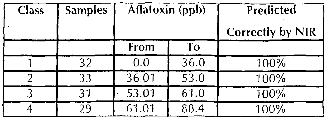
Class 1 (32 spectra corresponding to 0.0 - 36.0ppb aflatoxin) Class 2 (33 spectra corresponding to 36.01 - 53.0ppb aflatoxin) Class 3 (31 spectra corresponding to 53.01 - 61.0ppb aflatoxin) Class 4 (29 spectra corresponding to 61.01 - 88.4ppb aflatoxin) Groups were chosen not on aflatoxin concentration, but in a way such that each group had reasonably similar numbers of samples. As a general rule of thumb, hundreds of samples are usually required for calibration of each training set, depending on the difficultly in attaining the result range of the parameter of interest. Despite the limited sample numbers, a calibration model using the discriminate function, auto-baseline, cross validation and mean centring between 500-1 700nm was developed on each Class. An identification system containing 4 representative calibration models was therefore created, and all 125 "internal" validation spectra were taken and re-presented across the system; the end result being a Mahalanobis Distance (M) for each spectrum that describes the goodness of fit of the spectrum to each of the models. Class identification was confirmed as the lowest M Distance from each spectrum, and results summarised. Internal validations are used by the applicant to assess the capabilities of individual calibration models in terms of robustness and the ability to identify their own species accurately, before attempting detection of any external validation samples. Note: All internal val idation spectra were used in calibration development. The following table is a summary of prediction results for spectral data grouped into 4 classes according to aflatoxin concentration.

External validations were briefly tried by removal of random sample spectra from the training sets prior to calibration, but resulted in smaller calibration models that severely lacked robustness and prediction power. As results show, near-infrared spectroscopy worked brilliantly in this situation despite baseline aberrations, problems with particle size and ELISA test difficulties, producing a perfect result whereby all spectra used in the development calibrations were accurately identified. As another example, spectral data (see Appendix D) from each peanut meal sample was averaged to give a representative spectrum and paired with the corresponding ELISA test result before running several calibration models. A model using Partial Least Squares (PLS) with autobaseline, cross validation and mean centring between 400-1700nm attained R² = 0.478 and SECV= 15.93ppb with no outlier removal (see graph in Figure 9 showing the calibration model developed from 125 averaged spectra with no outlier removal using PLS, cross validation, mean centring, autobaseline and 400-1 700nm). A second model using similar parameters and all of the 1250 unaveraged spectra attained R² = 0.491 and SECV 1 5.64ppb with no outlier removal (see graph in Figure 10 showing the calibration model developed from 1 250 unaveraged spectra with no outlier removal using PLS, cross validation, mean centring, autobaseline and 400-1700nm). A further calibration removing 162 sample spectra from the concentration residual plot, that were predicting outside a 25ppb range, resulted in significantly better calibration statistics of R² = 0.656 and SECV = 1 1.43ppb (see graph in Figure 1 1 showing the calibration model developed from 1 250 unaveraged spectra after removal of 162 spectra that fell outside a 25ppb range on the concentration residual plot). Internal validation of averaged sample spectra across the latter model developed on unaveraged spectra produced aSEP = 27.68ppb for 95% of samples. This meant that 10 scans of a peanut meal could be taken, averaged and predicted to within 27.68ppb aflatoxin concentration and with 95%> confidence. Problems with Spectral Acquisition Peanut meal samples contain particles of uneven size and shape, relatively inappropriate for presentation to NIR spectroscopy at such close range. Ideally, spectra should deviate within reason to only the parameter of interest. Large spectral variations were due to these changes in particle size, rather than aflatoxin content. Since aflatoxin concentration ranged from 1.5ppb to around 9,0ppb, the minute spectral differences and fingerprints of aflatoxin Bl , B2, G1 & G2 would be largely masked by huge spectral differences in particle size.

APPENDIX A

(non-destructive prediction of apple TSS % juice in 20 Granny Smith apples run against a global apple TSS % juice calibration developed from laboratory data representing 10 apple varieties)

APPENDIX B

(non-destructive classification of 10 unknown apple spectra as Granny Smith apples; the unknown spectra run across 5 variety-specific apple calibration)

APPENDIX C

Sample OD Aflatoxin Cla; ample OD Aflatoxin Cla; ppb ppb 1 .268 88.4 4 63 .393 43.1 2 2 .273 86.1 4 64 .368 47.0 2 3 .289 79.6 4 65 .331 53.9 3 4 .284 81.5 4 66 .494 31.3 1 5 .272 86.6 4 67 .392 43.3 2 6 .270 87.5 4 68 .343 51.5 2 7 .277 84.4 4 69 .341 51.9 2 8 .290 79.2 4 70 .339 52.3 2 9 .297 76.6 4 71 .384 44.5 2 10 .302 74.8 4 72 .313 57.9 3 11 .304 74.1 4 73 .380 45.1 2 12 .298 76.2 4 74 .352 49.8 2 13 1.185 3.7 1 75 .896 14.2 1 14 .317 61.8 4 76 1.409 3.2 1 15 1.190 3.6 1 77 .334 61.0 4 16 1.336 1.6 1 78 .764 19.2 1 17 1.117 4.8 1 79 .699 22.4 1 18 1.087 5.4 1 80 .250 85.0 4 19 1.140 4.4 1 81 .383 51.7 2 20 1.180 3.7 1 82 .387 51.0 2 21 .334 57.5 3 83 .439 43.5 2 22 .356 52.6 3 84 .340 59.7 3 23 1.112 4.9 1 85 .518 35.0 1 24 1.176 3.8 1 86 .516 35.1 1 25 .296 56.0 3 87 .379 53.6 3 26 .262 64.7 4 88 .299 67.2 4 27 .321 50.7 2 89 .347 58.4 3 28 .317 51.5 2 90 .893 19.9 1 29 .286 58.3 3 91 1.303 9.8 1 30 .309 53.1 2 92 .974 17.4 1 31 .388 39.9 2 93 .642 30.6 1 32 .450 32.7 1 94 .590 33.8 1 33 .393 39.2 2 95 1.126 13.5 1 34 .344 46.5 2 96 .916 19.1 1 35 .316 51.7 2 97 .874 20.5 1 36 .340 49.6 2 98 .746 25.5 1 37 .269 68.0 4 99 .552 37.1 2 38 .295 60.1 3 100 .658 29.4 1 39 .354 46.8 2 101 .493 42.8 2 40 .299 59.1 3 102 .559 36.5 2 41 .344 48.8 2 103 .611 32.5 1 42 .312 55.8 3 104 .514 40.6 2 43 .287 62.4 4 105 .433 50.0 2 44 .993 6.8 1 106 .386 57.0 3 45 .294 60.4 3 107 .532 38.9 2 46 1.028 6.2 1 108 .526 39.5 2 47 1.038 6.0 1 109 .350 63.7 4 48 .318 57.4 3 110 .295 76.6 4 49 .287 65.3 4 111 .661 27.6 1 50 .297 62.6 4 112 .279 56.4 3 51 .284 66.2 4 113 .283 55.8 3 52 .283 66.5 4 114 .293 54.4 3 53 .289 64.8 4 115 .299 53.6 3

54 .351 50.5 2 116 .305 52.8 2

55 .309 59.5 3 117 .301 53.4 3

56 .316 57.8 3 118 .302 53.2 3

57 .317 57.6 3 119 .312 52.0 2

58 .306 60.3 3 120 .306 52.7 2

59 .291 64.2 4 121 .302 53.2 3

60 .321 56.7 3 122 .303 53.1 3

61 .253 76.4 4 123 .288 55.1 3

62 .265 72.2 4 124 .287 55.3 3 125 .296 54.0 3

APPENDIX D

Sample OD Aflatoxin Sampl OD Aflatoxin ppb e ppb 1 .268 88.4 63 .393 43.1 2 .273 86.1 64 .368 47.0 3 .289 79.6 65 .331 53.9 4 .284 81.5 66 .494 31.3 5 .272 86.6 67 .392 43.3 6 .270 87.5 68 .343 51.5 7 .277 84.4 69 .341 51.9 8 .290 79.2 70 .339 52.3 9 .297 76.6 71 .384 44.5 10 .302 74.8 72 .313 57.9 11 .304 74.1 73 .380 45.1 12 .298 76.2 74 .352 49.8 13 1.18 3.7 75 .896 14.2 5 14 .317 61.8 76 1.409 3.2 15 1.19 3.6 77 .334 61.0 0 16 1.33 1.6 78 .764 19.2 6 17 1.11 4.8 79 .699 22.4 7 18 1.08 5.4 80 .250 85.0 7 19 1.14 4.4 81 .383 51.7 0 20 1.18 3.7 82 .387 51.0 0 21 .334 57.5 83 .439 43.5. 22 .356 52.6 84 .340 59.7 23 1.11 4.9 85 .518 35.0 2 24 1.17 3.8 86 .516 35.1 6 25 .296 56.0 87 .379 53.6 26 .262 64.7 88 .299 67.2 27 .321 50.7 89 .347 58.4 28 .317 51.5 90 .893 19.9 29 .286 58.3 91 1.303 9.8

30 .309 53.1 92 .974 17.4

31 .388 39.9 93 .642 30.6

32 .450 32.7 94 .590 33.8

33 .393 39.2 95 1.126 13.5

34 .344 46.5 96 .916 19.1

35 .316 51.7 97 .874 20.5

36 .340 49.6 98 .746 25.5

37 .269 68.0 99 .552 37.1

38 .295 60.1 100 .658 29.4

39 .354 46.8 101 .493 42.8

40 .299 59.1 102 .559 36.5

41 .344 48.8 103 .611 32.5

42 .312 55.8 104 .514 40.6

43 .287 62.4 105 .433 50.0

44 .993 6.8 106 .386 57.0

45 .294 60.4 107 .532 38.9

46 1.02 6.2 108 .526 39.5 8

47 1.03 6.0 109 .350 63.7 8

48 .318 57.4 110 .295 76.6

49 .287 65.3 111 .661 27.6

50 .297 62.6 112 .279 56.4

51 .284 66.2 113 .283 55.8

52 .283 66.5 114 .293 54.4

53 .289 64.8 115 .299 53.6

54 .351 50.5 116 .305 52.8

55 .309 59.5 117 .301 53.4

56 .316 57.8 118 .302 53.2

57 .317 57.6 119 .312 52.0

58 .306 60.3 120 .306 52.7

59 .291 64.2 121 .302 53.2

60 .321 56.7 122 .303 53.1

61 .253 76.4 123 .288 55.1

62 .265 72.2 124 .287 55.3 125 .296 54.0 Whilst the above has been given by way of illustrative example of the present invention many variations and modifications thereto will be apparent to those skilled in the art without departing from the broad ambit and scope of the invention as herein set forth.

Claims

THE CLAIMS DEFINING THE INVENTION ARE AS FOLLOWS:

1. A system of calibrating spectra data for detecting substances including means for non-invasively acquiring a plurality of reflected spectra from each sample of a known substance; analysing means arranged to provide an averaged spectra data of the plurality of reflected spectra for each sample, and having one or more calibration models for analysing the spectra data to provide a comparison data, wherein the comparison data from the spectra data of the samples of known substances are for use as corresponding validation data sets, each set relating to the reflected spectra from the known substances of a specie; and storage means for storing the validation data sets.

2. A process of calibrating spectra data for detecting substances. The process includes the following steps: (1) non-invasively acquiring reflected spectra from a plurality of samples of a known substance; (2) averaging and validating acquired spectra from samples of the known substance to provide an averaged spectra data; (3) with a calibration model analysing the averaged spectra data to provide a comparison data, wherein the comparison data provided from averaged spectra data of known substances are for use as corresponding validation data sets, each set relating to the reflected spectra from known substances of a specie; and (4) storing the validation data sets in storage means;

3. An apparatus of acquiring spectra data for detecting substances including means for non-invasively acquiring reflected spectra froma substance; analysing means having one or more calibration models for analysing acquired spectra to provide a comparison data, wherein the comparison data provided from acquired spectra of known substances are for use as corresponding validation data sets, each set relating to the reflected spectra from known substances of a specie, and storage means for storing the validation data sets.