Abstract
We present the evolution of Lyα emission derived from 53 galaxies at z = 6.6–13.2, which have been identified by multiple JWST/NIRSpec spectroscopy programs of Early Release Science, General Observer, Director's Discretionary Time, and Guaranteed Time Observations. These galaxies fall on the star formation main sequence and are typical star-forming galaxies with UV magnitudes of −22.5 ≤ MUV ≤ −17.0. We find that 15 out of 53 galaxies show Lyα emission at the >3σ level, and we obtain Lyα equivalent width (EW) measurements and stringent 3σ upper limits for the 15 and 38 galaxies, respectively. Confirming that Lyα velocity offsets and line widths of our galaxies are comparable to those of low-redshift Lyα emitters, we investigate the redshift evolution of the Lyα EW. We find that Lyα EWs statistically decrease toward high redshifts on the Lyα EW versus the MUV plane for various probability distributions of the uncertainties. We then evaluate neutral hydrogen fractions xH I with the redshift evolution of the Lyα EW and the cosmic reionization simulation results on the basis of a Bayesian inference framework, and obtain xH I < 0.79,  , and
, and  at z ∼ 7, 8, and 9–13, respectively. These moderately large xH I values are consistent with the Planck cosmic microwave background optical depth measurement and previous xH I constraints from galaxy and QSO Lyα damping wing absorption and strongly indicate a late reionization history. Such a late reionization history suggests that major sources of reionization would emerge late and be hosted by moderately massive halos compared with the widely accepted picture of abundant low-mass objects for the sources of reionization.
Original content from this work may be used under the terms of the Creative Commons Attribution 4.0 licence. Any further distribution of this work must maintain attribution to the author(s) and the title of the work, journal citation and DOI.
1. Introduction
Cosmic reionization is a crucial phase transition in the early universe. During the epoch of reionization, the neutral hydrogen in the intergalactic medium (IGM) was ionized by UV photons emitted from the first sources. Fan et al. (2006) show that reionization is mainly completed by z ∼ 6 from the measurements of Gunn–Peterson troughs (Gunn & Peterson 1965) in the spectra of quasars (QSOs), while Kulkarni et al. (2019) suggest that a broad scatter in the neutral hydrogen fraction xH I exists at redshift as low as z ≲ 5.5. Thomson scattering optical depth to the cosmic microwave background (CMB) indicates that significant reionization occurred at z ∼ 7–8 (Planck Collaboration et al. 2020).
Reionization history is investigated by deriving the redshift evolution of xH I in the IGM. Lyα emission from star-forming galaxies is a good probe of xH i because the Lyα emission line is strongly attenuated by the neutral hydrogen via the Lyα damping wing (Ouchi et al. 2020). While Lyα emitters (LAEs) have been commonly found at z ≃ 6 (e.g., Stark et al. 2011; De Barros et al. 2017), LAEs at higher redshift z ≳ 7 are rare (e.g., Stark et al. 2010; Treu et al. 2013; Hoag et al. 2019; Jung et al. 2020). Although reionization history is constrained by many studies of LAE clustering analysis (e.g., Ouchi et al. 2018; Umeda 2023), Lyα luminosity function (e.g., Ouchi et al. 2010; Konno et al. 2014; Hu et al. 2019; Wold et al. 2022), and Lyα equivalent width (EW) distribution (e.g., Mason et al. 2018; Hoag et al. 2019; Bolan et al. 2022), the uncertainties of reionization history are still large at z ∼ 6–8. At a higher redshift of z ≳ 8, almost no observational constraints existed before the arrival of the James Webb Space Telescope (JWST; Ferruit et al. 2022; Jakobsen et al. 2022; Böker et al. 2023; Gardner et al. 2023; Rieke et al. 2023; Rigby et al. 2023). JWST allows a deep survey of faint galaxies during the epoch of reionization. In fact, many LAEs are spectroscopically identified at a high redshift of 7 ≲ z ≲ 11 (e.g., Bunker et al. 2023b; Jung et al. 2023; Tang et al. 2023; Chen et al. 2024; Jones et al. 2024; Saxena et al. 2024). In addition, recent studies of JWST observations place the constraints on reionization history at z ≳ 8 (Hsiao et al. 2023; Curtis-Lake et al. 2023; Umeda et al. 2023), although the constraints are not strong. The open questions regarding reionization are thus when reionization started and at what pace reionization proceeded.
Lyα EW, defined by a Lyα flux relative to a UV continuum flux, is a key observable property that reflects the intensity of the Lyα emission. The fraction of LAEs (EW > 25Å) among Lyman-break galaxies (LBGs), the Lyα fraction, is measured as a way to put a constraint on the Lyα optical depth (e.g., Stark et al. 2010; Ono et al. 2012; Schenker et al. 2012; Treu et al. 2012; Pentericci et al. 2018; Jones et al. 2024). The Lyα fraction dramatically decreases from z ∼ 6 to 7, indicating the rapid increase in Lyα optical depth at z ≳ 6. Treu et al. (2012, 2013) suggest that the full Lyα EW distribution, including galaxies with low Lyα EW and no Lyα detections, contains more information about the Lyα optical depth than the Lyα fraction, which is used to evaluate the fraction of galaxies detected at some fixed threshold of Lyα EW. The xH I values in the IGM are not directly constrained by the Lyα optical depth because Lyα photons are absorbed by the neutral hydrogen not only in the IGM, but also in the interstellar medium (ISM) and circumgalactic medium (CGM). The effects of the ISM and CGM on Lyα transmission have been studied by some models or simulations (e.g., Dijkstra et al. 2011; Mesinger et al. 2015). Mason et al. (2018) introduce a flexible Bayesian framework based on that of Treu et al. (2012, 2013) and the simulations by Mesinger et al. (2015) to infer xH I from LBGs with detections and no detections of Lyα emission.
The source of reionization is another important feature of reionization. Recent observational studies report a steep faint-end slope α of a UV luminosity function (Bouwens et al. 2017; Livermore et al. 2017; Atek et al. 2018; Ishigaki et al. 2018; Finkelstein et al. 2019), indicating that faint sources make dominant contributions to UV luminosity correlated with ionizing photon production. Although the escape fraction of ionizing photons fesc is also crucial to understanding ionizing sources, it is impossible to directly measure fesc at z > 4, due to the high optical depth of ionizing photons (e.g., Vanzella et al. 2018). In addition, recent works of simulations and semi-analytical models show conflicting results for fesc correlated with halo mass (e.g., Gnedin et al. 2008; Wise & Cen 2009; Sharma et al. 2016) and anticorrelated with halo mass (e.g., Paardekooper et al. 2015; Faisst 2016; Kimm et al. 2017). The fesc value during the epoch of reionization thus remains uncertain. However, given that low-mass (massive) galaxies contribute to early (late) reionization (e.g., Faisst 2016; Dayal et al. 2024), we may be able to constrain the mass dependence of reionization source from reionization history.
There are three scenarios of the reionization history suggested by Naidu et al. (2020), Ishigaki et al. (2018), and Finkelstein et al. (2019), referred to as the late scenario, medium-late scenario, and early scenario, respectively. The three scenarios differ in the escape fraction of ionizing photons fesc and the faint-end slope α of the UV luminosity function. We refer to Model II described in Naidu et al. (2020) as the late scenario because Model II self-consistently explains observational results of the redshift evolution of fesc (e.g., Siana et al. 2010; Rutkowski et al. 2016; Marchi et al. 2017; Steidel et al. 2018; Fletcher et al. 2019). In the late scenario, the faint-end slope should be shallow (α > −2) with the assumption that fesc depends on the star formation rate (SFR) surface density ΣSFR. Bright and massive galaxies (MUV < −18 and stellar mass M* > 108 M⊙) are major contributors to reionization in this scenario. In the medium-late scenario, Ishigaki et al. (2018) find the steep faint-end slope (α ≲ −2) from observations and the constant escape fraction (fesc ∼ 0.17) with which the scenario can mostly explain the observational measurements. Galaxies with various luminosities contribute to reionization in this scenario. In the early scenario, the faint-end slope should be steep (α ≲ −2) with the assumption that fesc anticorrelates with halo mass Mh. Faint and low-mass galaxies (MUV > −15 and M* ≲ 106 M⊙) are major contributors to reionization in this scenario.
In this study, we present the evolution of Lyα emission with 53 galaxies at z ≳ 7 whose redshifts are spectroscopically confirmed by JWST/NIRSpec. Combining these high-redshift galaxies and the full distributions of Lyα EW with detections and upper limits, we infer xH I at z ∼ 7–13. The xH I values provide insights into reionization history and sources. This paper is constructed as follows. Section 2 describes the JWST/NIRSpec spectroscopic data and our sample of galaxies. We conduct spectral fittings to our sample galaxies and investigate the Lyα properties obtained from the best-fit parameters in Section 3. In Section 4, we explain our method to infer xH I and present the estimated xH I values. In Section 5, we discuss reionization history and sources. Section 6 summarizes our findings. Throughout this paper, we use a standard ΛCDM cosmology with ΩΛ = 0.7, Ωm = 0.3, and H0 = 70 km s−1 Mpc−1. All magnitudes are in the AB system (Oke & Gunn 1983).
2. Data and Sample
The spectroscopic data sets used in this study were obtained in multiple public observation programs: the Early Release Science (ERS) observations of GLASS (ERS-1324, PI: T. Treu; Treu et al. 2022) and the Cosmic Evolution Early Release Science (CEERS; ERS-1345, PI: S. Finkelstein; Arrabal Haro et al. 2023a; Finkelstein et al. 2023), General Observer (GO) observations (GO-1433, PI: D. Coe; Hsiao et al. 2023), the Directors Discretionary Time (DDT) observations (DDT-2750, PI: P. Arrabal Haro; Arrabal Haro et al. 2023b), and the Guaranteed Time Observations (GTO) of the JWST Advanced Deep Extragalactic Survey (JADES; GTO-1210, PI: N. Lützgendorf; Bunker et al. 2023a; Eisenstein et al. 2023). The GLASS data were taken at one pointing position with high resolution (R ∼ 2700) filter-grating pairs of F100LP-G140H, F170LP-G235H, and F290LP-G395H covering the wavelength ranges of 1.0–1.6, 1.7–3.1, and 2.9–5.1 μm, respectively. The total exposure time of the GLASS data is 4.9 hr for each filter-grating pair. The CEERS data were taken at 8 and 6 pointing positions with the prism (R ∼ 100) and medium-resolution grating (R ∼ 1000), respectively. The prism covered the wavelength of 0.6–5.3 μm. The filter-grating pairs of medium-resolution grating observations were F100LP-G140M, F170LP-G235M, and F290LP-G395M, whose wavelength coverages were 1.0–1.6, 1.7–3.1 and 2.9–5.1 μm, respectively. The total exposure time of the CEERS data is 0.86 hr for each filter-grating pair per pointing. The GO-1433 and DDT-2750 observations, each at a single pointing, were conducted with the prism, and the total exposure times are 3.7 and 5.1 hr, respectively. The JADES data were obtained at 3 pointing positions with the prism and four filter-grating pairs of F070LP-G140M (0.7–1.3 μm), F170LP-G235M, F290LP-G395M, and F290LP-G395H. The total exposure times of the JADES observations are 9.3 hr for the prism and 2.3 hr for each filter-grating pair per pointing. Nakajima et al. (2023) and Harikane et al. (2024) have reduced the GLASS, CEERS, GO-1433, and DDT-2750 data with the JWST pipeline version 1.8.5 with the Calibration Reference Data System context file of jwst_1028.pmap or jwst_1027.pmap with additional processes improving the flux calibration, noise estimate, and the composition, and have measured systemic redshifts zsys with optical emission lines (Hβ, [O iii]λ4959, and [O iii]λ5007). See Nakajima et al. (2023) and Harikane et al. (2024) for further details of the data reduction and zsys determination. The combination of the data of Nakajima et al. (2023) and Harikane et al. (2024) from the public observational programs provides a sample of 196 galaxies at 4.0 ≤ zsys ≤ 11.4. We then select 35 galaxies with zsys ≥ 7 from the sample that is referred to as the public data sample. The JADES data are publicly available, 7 and have already been reduced with the pipeline developed by the ESA NIRSpec Science Operations Team and the NIRSpec GTO Team. The JADES data consists of 178 galaxies at 0.7 ≤ zsys ≤ 13.2, including 75 galaxies whose redshifts are undetermined. We select 18 galaxies from the JADES data with zsys ≥ 6.5 identified by Bunker et al. (2023a) with emission lines (e.g., Hβ, [O iii]λ4959, and [O iii]λ5007) or spectral breaks. To these 18 galaxies, we add GN-z11 at zsys = 10.6, which is also observed as part of the JADES program (GTO-1181, PI: D. Eisenstein; Eisenstein et al. 2023). We refer to a total of these 19 galaxies as the JADES data sample. Note that we use the values of the rest-frame Lyα EW, Lyα velocity offset, and line width presented in the literature (Bunker et al. 2023b). Combining the JADES data sample with the public data sample, we obtain a total of 54 galaxies whose zsys fall in the range of 6.6 ≤ zsys ≤ 13.2. Here, 6, 26, 1, 2, and 19 out of all 54 galaxies are found in the GLASS, CEERS, GO-1433, DDT-2750, and JADES data, respectively. We note that these 54 galaxies in the public data and JADES data samples are observed with the gratings and/or prism. The public data sample (35 galaxies) consists of 17, 26, and 8 galaxies that have the grating, prism, and grating+prism spectra, respectively. The JADES data sample (19 galaxies) has both the grating and prism spectra, while the grating spectra at the Lyα wavelengths are missing in three galaxies. There are a total of 33 (=17 + 19 −3) galaxies whose Lyα emission wavelengths are observed with the gratings. The rest of the objects, 21 (=54–33) galaxies, have only the prism spectra, where the measurements of the Lyα velocity offset and line width are not obtained due to the poor spectral resolution.
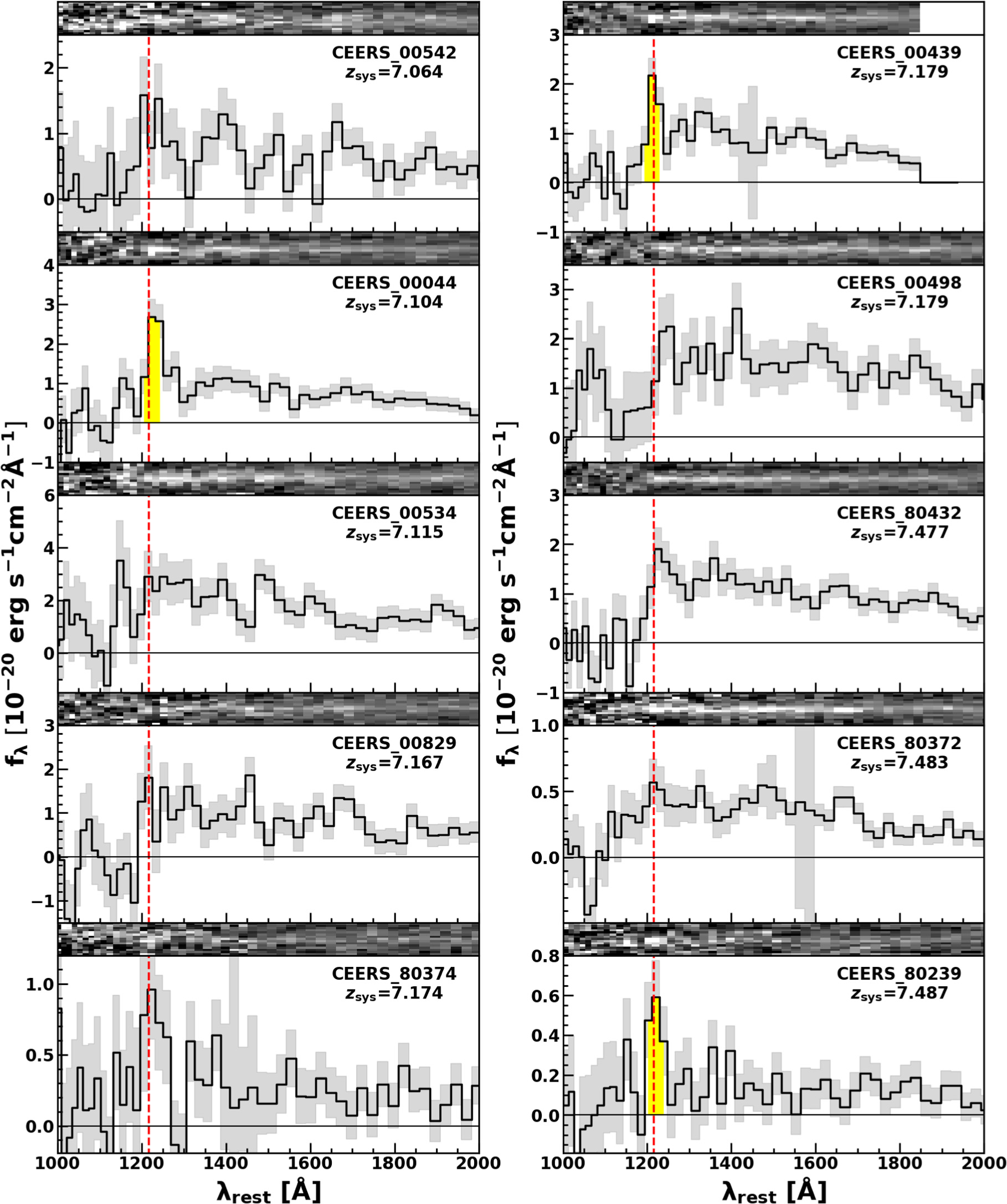
In Figures 1 and 2, we show the spectra of 53 galaxies with the exception of GN-z11. We note that because CEERS_01027 is observed at two pointing positions with the medium-resolution grating, two spectra of CEERS_01027 (CEERS_P4M_01027 and CEERS_P10M_01027) are shown in Figure 1.
Download figure:
Standard image High-resolution image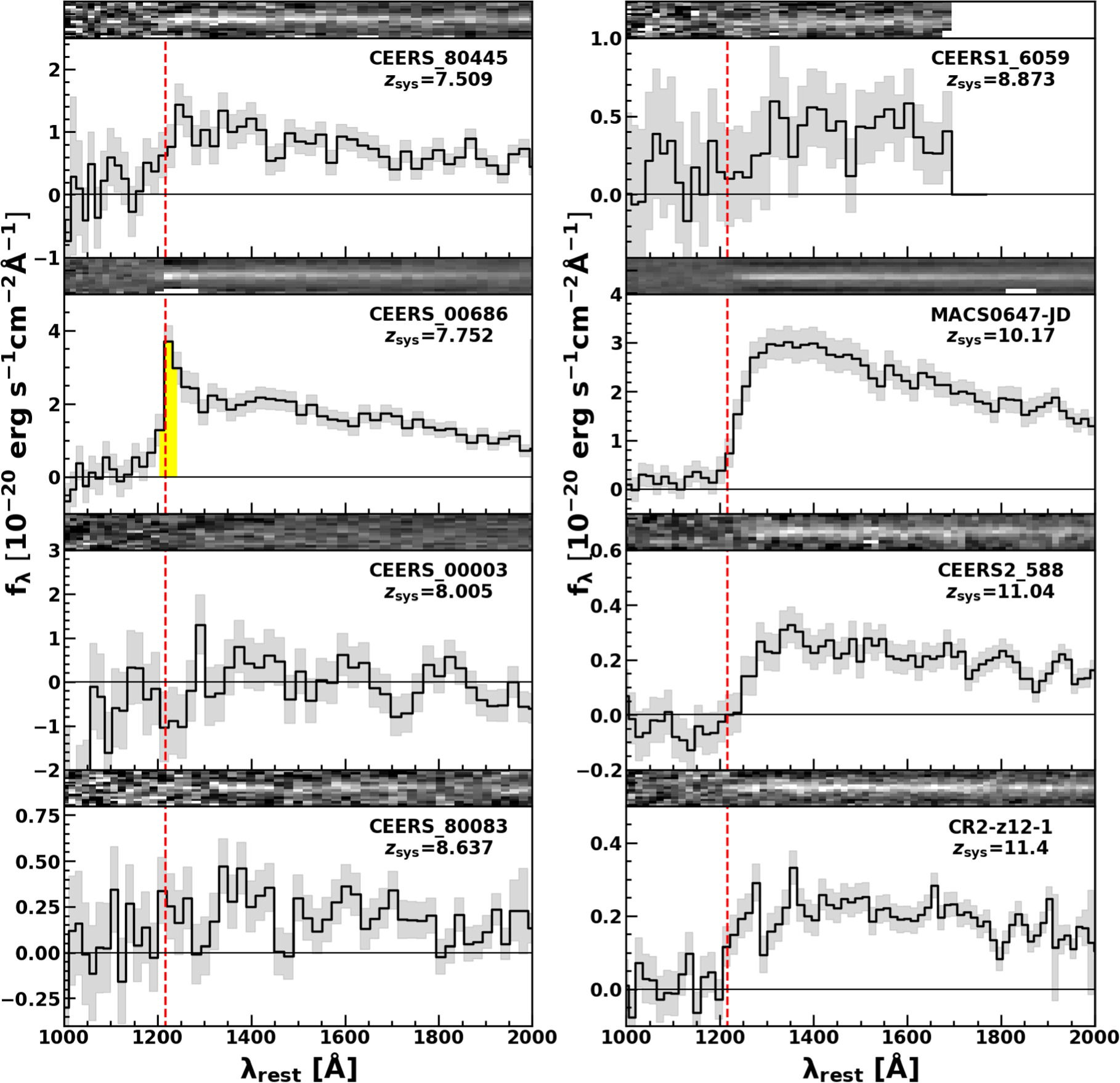
Download figure:
Standard image High-resolution image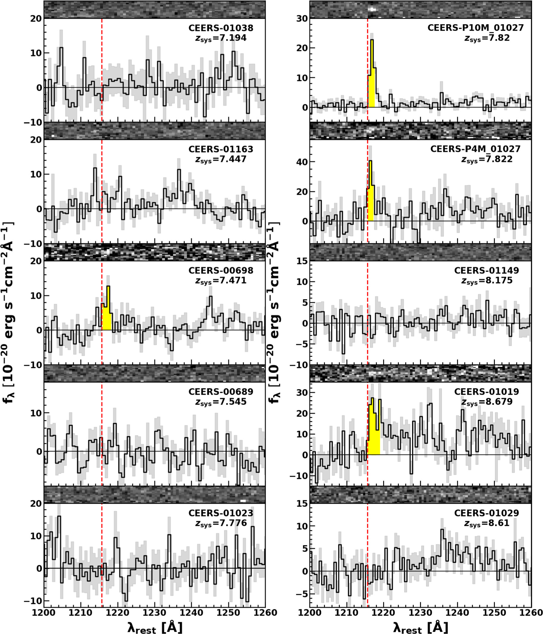
Download figure:
Standard image High-resolution image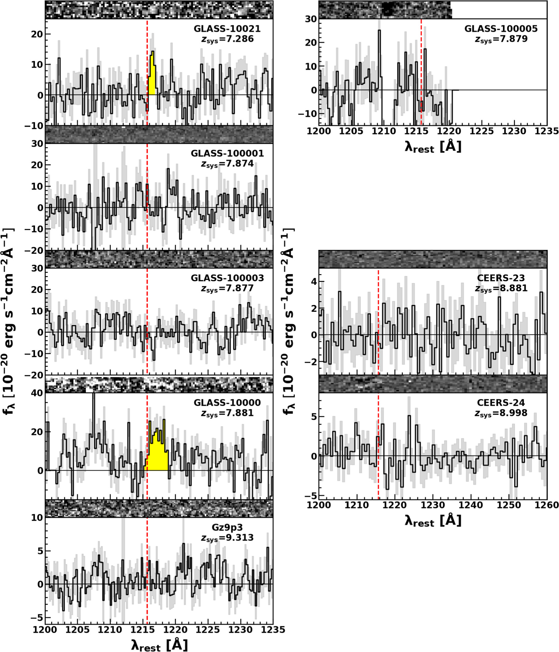
Figure 1. Spectra of the public data sample. Each panel shows the two-dimensional spectrum (top) and the one-dimensional spectrum (bottom). The black solid lines and shaded regions represent the observed spectra and associated 1σ errors, respectively. The vertical red-dashed lines represent the rest-frame Lyα wavelengths of 1215.67 Å at the systemic redshifts. The yellow regions indicate the detected Lyα lines whose signal-to-noise ratio is larger than 3σ (Section 3.1).
Download figure:
Standard image High-resolution image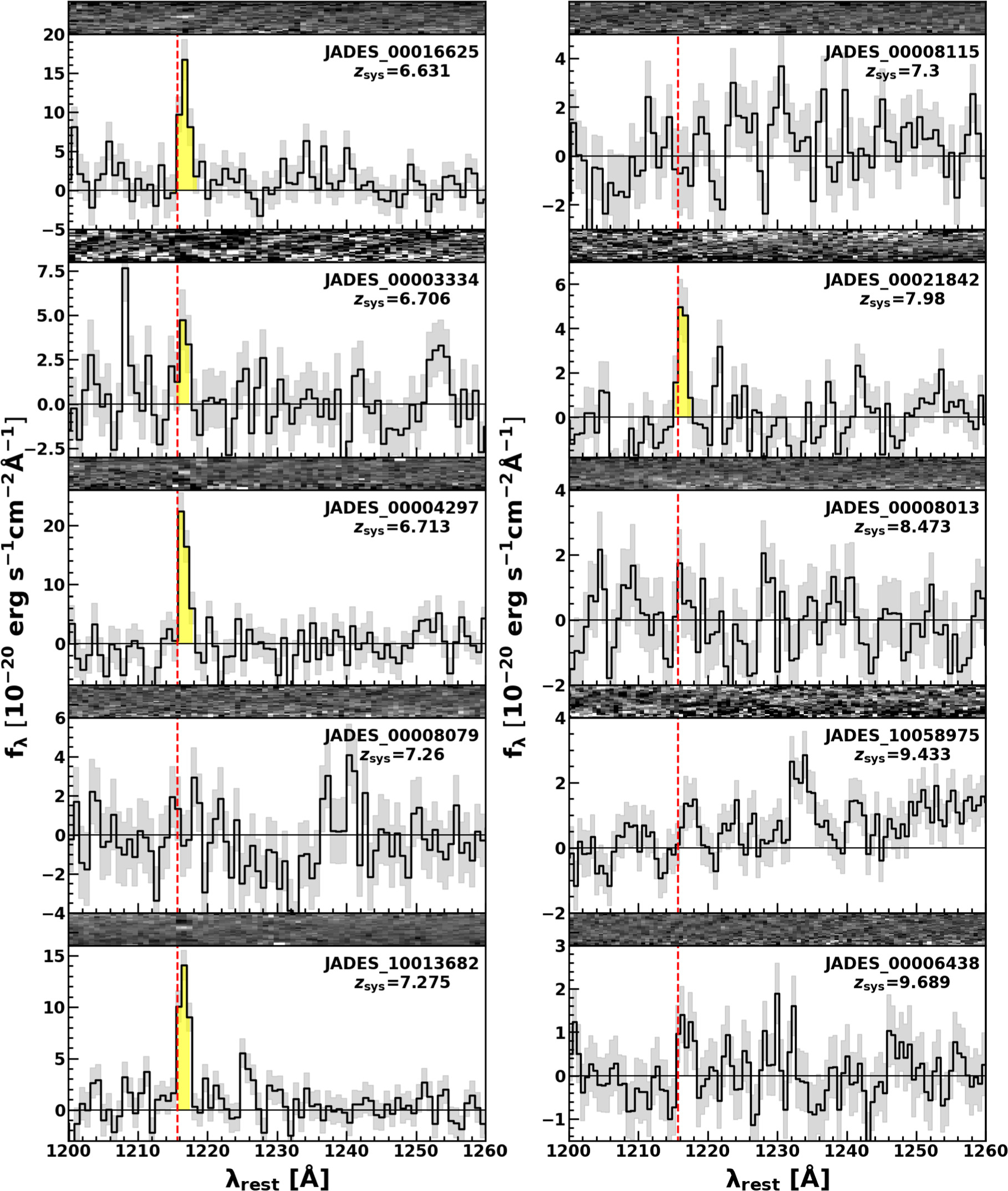
Download figure:
Standard image High-resolution image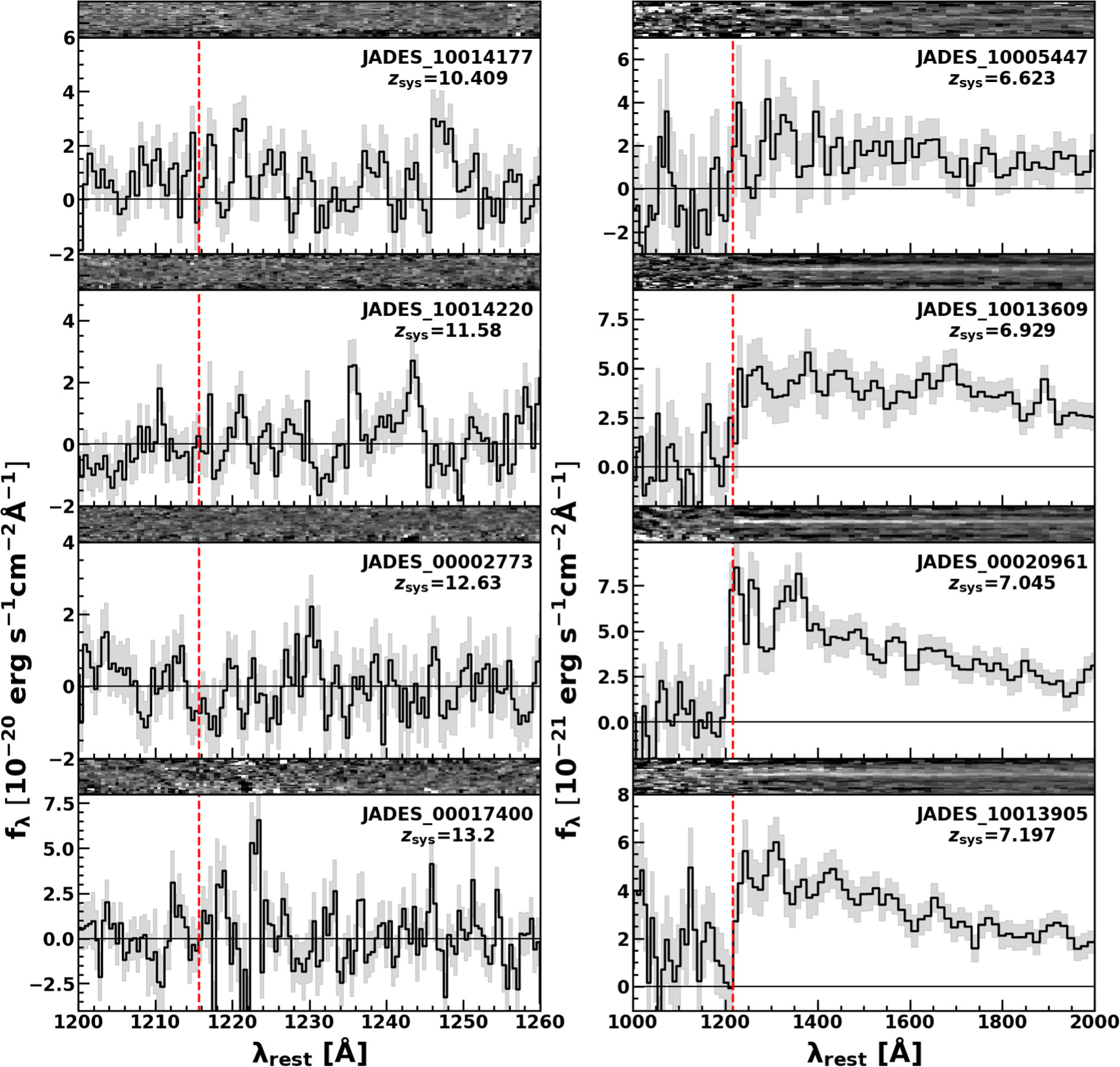
Figure 2. Same as Figure 1, but for the JADES data sample.
Download figure:
Standard image High-resolution imageIn Figure 3, we compare the stellar mass M* and SFR of our galaxies with those of the star formation main sequence (MS) to confirm whether our galaxies are typical star-forming galaxies or not. We adopt the stellar mass and SFR reported by Nakajima et al. (2023) and Harikane et al. (2024) for 14 and 5 galaxies of the public data sample, respectively. We use the stellar mass and SFR reported by Curti et al. (2024), Harikane et al. (2024), and Bunker et al. (2023b) for 11, 3, and 1 galaxies of the JADES data sample, respectively. For 11 galaxies for which Nakajima et al. (2023) only report the stellar mass estimates, we calculate the SFR from the UV magnitude. We first derive the UV luminosity Lν (UV) from the UV magnitude. We then convert the UV luminosity into the SFR with SFR = 1.15 × 10⁻²⁸ Lν (UV) (Madau & Dickinson 2014). We correct the SFR for the dust extinction, using an extinction−UV slope βUV relation (Meurer et al. 1999) and βUV–MUV relation (Bouwens et al. 2014). In Figure 3, we do not present the other nine galaxies whose stellar mass is not determined. The stellar masses and SFRs of our galaxies are comparable with the star formation MSs at z ∼ 6 (Santini et al. 2017), indicating that our galaxies are typical star-forming galaxies.

Figure 3. SFR as a function of stellar mass. The red squares and orange circles present our sample galaxies whose SFRs are measured in this work and the literature (Bunker et al. 2023b; Nakajima et al. 2023; Curti et al. 2024; Harikane et al. 2024), respectively. The blue solid line and shaded region indicate the star formation MS at z ∼ 6 and its uncertainty (Santini et al. 2017), respectively.
Download figure:
Standard image High-resolution image3. Measurements of Lyα Fluxes and the Properties
3.1. Spectral Fitting
To obtain the Lyα emission properties of galaxies, we fit a continuum+line model to the Lyα emission line. This model is the linear combination of power-law a
λ−β
and Gaussian ![$A\exp \left[-{\left(\lambda -{\lambda }_{\mathrm{cen}}\right)}^{2}/{\sigma }^{2}\right]$](https://content.cld.iop.org/journals/0004-637X/967/1/28/revision1/apjad38c2ieqn3.gif) functions, where a, β, A, λcen, and σ are the free parameters. This model is multiplied by
functions, where a, β, A, λcen, and σ are the free parameters. This model is multiplied by ![$\exp \left[-\tau \left(\lambda \right)\right]$](https://content.cld.iop.org/journals/0004-637X/967/1/28/revision1/apjad38c2ieqn4.gif) , where τ(λ) is the optical depth of the IGM to the Lyα photons at the observed wavelength λ (Inoue et al. 2014). We then convolve the model with the line spread functions (LSF) of JWST/NIRSpec measured with a spectrum of a planetary nebula (Isobe et al. 2023a) to account for instrumental smoothing.
, where τ(λ) is the optical depth of the IGM to the Lyα photons at the observed wavelength λ (Inoue et al. 2014). We then convolve the model with the line spread functions (LSF) of JWST/NIRSpec measured with a spectrum of a planetary nebula (Isobe et al. 2023a) to account for instrumental smoothing.
We determine the free parameters of the model, using emcee (Foreman-Mackey et al. 2013) to conduct Markov Chain Monte Carlo (MCMC) simulations. We apply this fitting method to the prism spectra of galaxies in the public data sample. For both the grating and prism spectra of galaxies in the JADES data sample, we add the full width at half-maximum (FWHM) for the LSF as an additional free parameter. Because the spectral resolution of the JADES data sample is higher than those of the other spectra due to the compact morphologies of the JADES targets (Jones et al. 2024), differences in the FWHM for the LSF have an influence on the fittings. The signal-to-noise ratio of the continua in the grating spectra of our galaxies is worse than that in the prism spectra, which do not allow us to simultaneously determine the amplitude a and the slope β of the power law. We thus fix the slope of the power law to zero for the grating spectra under the assumption of a flat continuum (fν = const.), which is typical for star-forming galaxies (Stark et al. 2010), and determine the rest of the model parameters. We show examples of the posterior distributions of the fitting parameters in Figure 4. We determine the model parameter and 1σ uncertainty by the mode (i.e., a peak of the posterior distribution) and 68th percentile highest posterior density interval (HPDI; i.e., the narrowest interval containing 68%) of the posterior distribution, respectively, which are good representatives even for a skewed posterior distribution. We are not able to conduct spectral fittings to the grating spectra of JADES_10013905 and GLASS_100005 due to the small numbers of spectral pixels on the redder side than the observed Lyα wavelengths. As for JADES_10013905, we use the prism spectrum for the fitting.
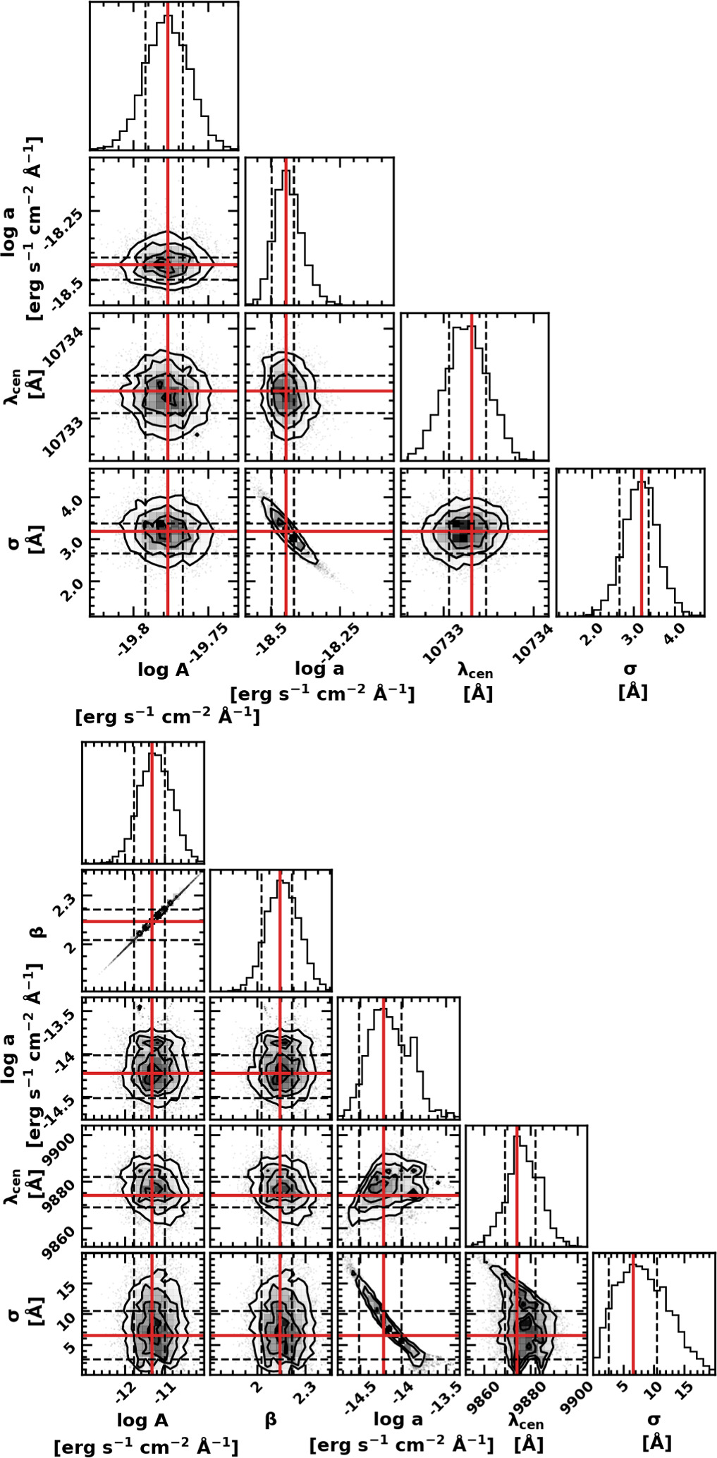
Figure 4. The posterior probability distribution functions of the fitting parameters. The top (bottom) panel presents the fitting results for a grating (prism) spectrum of CEERS-P10M_01027 (CEERS_00439). The red solid lines and black-dashed lines show the mode and the boundaries of the 68th percentile HPDI, respectively (Section 3.1).
Download figure:
Standard image High-resolution imageIn summary, we conducted spectral fittings to the grating spectra of 30 (=33 −2 −1) galaxies (not including GNz-11) and the prism spectra of 22 (=21 + 1) galaxies (see Section 2). Note that we have detected continua for 52 (=30 + 22) galaxies, including tentative detections. We confirm that if we use galaxies with continua detected at the >3σ level for the analysis below, our results do not change significantly.
With the public data and JADES data samples, we find that 11 out of 31 galaxies with the grating spectra and four out of 22 galaxies with the prism spectra have Lyα detections, where we place a threshold of the signal-to-noise ratio of >3σ for Lyα detection. In total, we find 15 (=11 + 4) out of 53 galaxies with Lyα detections in our sample. We note that Lyα emission of CEERS_01029 is not detected beyond our threshold, while Tang et al. (2023) claim the detection of Lyα emission. However, we confirm that the Lyα EW measurements of Tang et al. (2023), EW0,Lyα = 4.2 ± 1.3 Å, is within the 3σ upper limits of the Lyα EW in this work, 9.8 Å.
Table 1 summarizes the properties of all 54 galaxies in our sample. Table 2 compares the rest-frame Lyα EW and Lyα velocity offset of the galaxies, with Lyα detections measured in this study with those in the literature. For CEERS_01027, we show mean values of the Lyα redshift, EW, velocity offset, and line width measured from two grating spectra (Section 2) because the measurements from the two spectra are consistent within errors.
Table 1. Sample in This Study
| Name | zsys | zLyα | MUV | EW0,Lyα | ΔvLyα | FWHM |

| logSFR | References |
|---|---|---|---|---|---|---|---|---|---|
| (mag) | (Å) | (km s−1) | (km s−1) | (M⊙) | (M⊙ yr−1) | ||||
| (1) | (2) | (3) | (4) | (5) | (6) | (7) | (8) | (9) | (10) |
| JADES_10005447 | 6.623 (line) | ⋯ | −17.61 | <60.9 a | ⋯ | ⋯ |

|

| (5, 7, 11) |
| JADES_00016625 b | 6.631 (line) | 6.637 | −18.76 | 26.6 ± 7.1 | 234 ± 31 | 408 ± 110 |

|

| (5, 7, 11) |
| JADES_00003334 b | 6.706 (line) | 6.712 | −17.96 | 16.5 ± 4.2 | 229 ± 113 | 207 ± 128 |

|

| (5, 7, 11) |
| JADES_00004297 b | 6.713 (line) | 6.718 | −18.51 | 36.6 ± 5.0 | 188 ± 54 | 447 ± 60 |

|

| (5, 7, 11) |
| JADES_10013609 | 6.929 (line) | ⋯ | −18.69 | <1.9 a | ⋯ | ⋯ |

|

| (5, 7, 11) |
| JADES_00020961 | 7.045 (line) | ⋯ | −18.84 | <12.2 a | ⋯ | ⋯ |

|

| (5, 7, 11) |
| CEERS_00542 | 7.064 (line) | ⋯ | −19.89 | <47.6 a | ⋯ | ⋯ |

|

| (This work, 14) |
| CEERS_00044 | 7.104 (line) | ⋯ | −19.38 | 62.6 ± 19.5 a | ⋯ | ⋯ |

|

| (This work, 14) |
| CEERS_00534 | 7.115 (line) | ⋯ | −20.10 | <35.3 a | ⋯ | ⋯ |

|

| (This work, 14) |
| CEERS_00829 | 7.167 (line) | ⋯ | −19.57 | <41.3 a | ⋯ | ⋯ |

|

| (This work, 14) |
| CEERS_80374 | 7.174 (line) | ⋯ | −18.09 | <86.7 a | ⋯ | ⋯ |

|

| (This work, 14) |
| CEERS_00439 | 7.179 (line) | ⋯ | −19.28 | 33.8 ± 8.0 a | ⋯ | ⋯ |

|

| (This work, 14) |
| CEERS_00498 | 7.179 (line) | ⋯ | −20.20 | <30.6 a | ⋯ | ⋯ |

|

| (This work, 14) |
| CEERS_01038 | 7.194 (line) | ⋯ | −19.24 | <9.1 | ⋯ | ⋯ |

|

| (14) |
| JADES_10013905 | 7.197 (line) | ⋯ | −18.80 | <7.2 a , c | ⋯ | ⋯ |

|

| (5, 7) |
| JADES_00008079 | 7.260 (line) | ⋯ | −17.95 | <8.2 | ⋯ | ⋯ | ⋯ | ⋯ | (5, 11) |
| JADES_10013682 b | 7.275 (line) | 7.281 | −17.00 | 31.5 ± 3.3 | 215 ± 23 | 261 ± 57 |

|

| (5, 7, 11) |
| GLASS_10021 | 7.286 (line) | 7.292 | −21.44 | 3.2 ± 1.0 | 203 ± 32 | 121 ± 72 |

|

| (14) |
| JADES_00008115 | 7.3 (break) | ⋯ | ⋯ | <4.3 | ⋯ | ⋯ | ⋯ | ⋯ | (5) |
| CEERS_01163 | 7.455 (line) | ⋯ | > −20.78 | <9.3 | ⋯ | ⋯ | <8.98 | ⋯ | (14) |
| CEERS_00698 b | 7.471 (line) | 7.480 | −21.60 | 5.4 ± 1.0 | 334 ± 64 | 354 ± 135 |

|

| (14) |
| CEERS_80432 | 7.477 (line) | ⋯ | −20.05 | <27.3 a | ⋯ | ⋯ |

|

| (This work, 14) |
| CEERS_80372 | 7.483 (line) | ⋯ | −19.27 | <34.5 a | ⋯ | ⋯ |

|

| (14) |
| CEERS_80239 | 7.487 (line) | ⋯ | −17.92 | 105.3 ± 24.0 a | ⋯ | ⋯ |

|

| (14) |
| CEERS_80445 | 7.509 (line) | ⋯ | −19.66 | <18.2 a | ⋯ | ⋯ |

|

| (This work, 14) |
| CEERS_00689 | 7.552 (line) | ⋯ | −21.98 | <8.3 | ⋯ | ⋯ | <8.70 | ⋯ | (12, 14) |
| CEERS_00686 | 7.752 (line) | ⋯ | −20.68 | 20.4 ± 6.6 a | ⋯ | ⋯ | <8.44 | ⋯ | (12, 14) |
| CEERS_01023 | 7.776 (line) | ⋯ | −21.06 | <17.5 | ⋯ | ⋯ |

|

| (14) |
| CEERS_01027 b , d | 7.821 (line) | 7.828 | −20.73 | 17.9 ± 2.5 | 232 ± 56 | 283 ± 57 |

|

| (14) |
| GLASS_100001 | 7.874 (line) | ⋯ | −20.29 | <16.7 | ⋯ | ⋯ |

|

| (14) |
| GLASS_100003 | 7.877 (line) | ⋯ | −20.69 | <0.2 | ⋯ | ⋯ |

|

| (14) |
| GLASS_100005 | 7.879 (line) | ⋯ | −20.06 | ⋯ c | ⋯ | ⋯ |

|

| (14) |
| GLASS_10000 | 7.881 (line) | 7.890 | −20.36 | 7.5 ± 1.3 | 308 ± 102 | 818 ± 250 |

|

| (14) |
| JADES_00021842 b | 7.980 (line) | 7.985 | −18.71 | 18.8 ± 4.9 | 168 ± 91 | 277 ± 115 |

|

| (5, 7, 11) |
| CEERS_00003 | 8.005 (line) | ⋯ | −18.76 | <186.3 a | ⋯ | ⋯ |

|

| (This work, 14) |
| CEERS_01149 | 8.184 (line) | ⋯ | −20.83 | <11.8 | ⋯ | ⋯ |

|

| (14) |
| JADES_00008013 | 8.473 (line) | ⋯ | −17.54 | <6.0 | ⋯ | ⋯ |

|

| (5, 7, 11) |
| CEERS_01029 | 8.615 (line) | ⋯ | −21.14 | <9.8 | ⋯ | ⋯ |

|

| (This work, 14) |
| CEERS_90671 | 8.637 (line) | ⋯ | −18.7 | <45.2 a | ⋯ | ⋯ |

|

| (2, 9, 14) |
| CEERS_01019 | 8.679 (line) | 8.686 | −22.44 | 3.4 ± 1.1 | 231 ± 54 | 978 ± 248 |

|

| (9, 13, 17) |
| (14, 15, 16) | |||||||||
| CEERS1_6059 | 8.873 (line) | ⋯ | −20.75 | <14.3 a | ⋯ | ⋯ |

|

| (8, 9, 14) |
| CEERS-23 | 8.881 (line) | ⋯ | −18.9 | <21.7 | ⋯ | ⋯ |

|

| (8, 9, 16) |
| CEERS-24 | 8.998 (line) | ⋯ | −19.4 | <22.7 | ⋯ | ⋯ |

|

| (8, 9, 16) |
| Gz9p3 | 9.313 (line) | ⋯ | −21.6 | <2.3 | ⋯ | ⋯ | ⋯ | ⋯ | (3, 9) |
| JADES_10058975 | 9.433 (line) | ⋯ | −20.36 | <0.7 | ⋯ | ⋯ |

|

| (5, 7, 11) |
| JADES_00006438 | 9.689 (line) | ⋯ | −19.27 | <17.7 | ⋯ | ⋯ | ⋯ | ⋯ | (5, 11) |
| MACS0647-JD | 10.17 (line) | ⋯ | −20.3 | <5.9 a | ⋯ | ⋯ | ⋯ | ⋯ | (9, 10) |
| JADES_10014177 | 10.409 (break) | ⋯ | −18.45 | <4.2 | ⋯ | ⋯ | ⋯ | ⋯ | (11) |
| GN-z11 | 10.603 (line) | 10.624 | −21.5 | 18.0 ± 2.0 | 555 ± 32 | 566 ± 61 |

|

| (4) |
| CEERS2_588 | 11.04 (line) | ⋯ | −20.4 | <11.5 a | ⋯ | ⋯ |

|

| (9) |
| CR2-z12-1 | 11.40 (line) | ⋯ | −20.1 | <9.4 a | ⋯ | ⋯ |

|

| (1, 9) |
| JADES_10014220 | 11.58 (break) | ⋯ | −19.36 | <2.3 | ⋯ | ⋯ |

|

| (5, 6, 9) |
| JADES_00002773 | 12.63 (break) | ⋯ | −18.8 | <5.8 | ⋯ | ⋯ |

|

| (5, 6, 9) |
| JADES_00017400 | 13.20 (break) | ⋯ | −18.5 | <3.8 | ⋯ | ⋯ |

|

| (5, 6, 9) |
Notes. Columns: (1) Name. (2) Systemic redshift. The spectroscopic feature used to determine the redshift is noted (break: Lyman break, line: emission line). (3) Lyα redshift. (4) Absolute UV magnitude. (5) Rest-frame Lyα EW and the 1σ error. For galaxies with no Lyα detections, we show 3σ upper limits. (6) Lyα velocity offset. (7) FWHM of the Lyα emission line. (8) Stellar mass. (9) SFR.
References. For systemic redshifts, absolute UV magnitude, stellar masses, and SFRs. This work, (1) Arrabal Haro et al. (2023a), (2) Arrabal Haro et al. (2023b), (3) Boyett et al. (2024), (4) Bunker et al. (2023b), (5) Bunker et al. (2023a), (6) Curtis-Lake et al. (2023), (7) Curti et al. (2024), (8) Fujimoto et al. (2023), (9) Harikane et al. (2024), (10) Hsiao et al. (2023), (11) Jones et al. (2024), (12) Jung et al. (2023), (13) Larson et al. (2023), (14) Nakajima et al. (2023), (15) Sanders et al. (2023), (16) Tang et al. (2023), (17) Zitrin et al. (2015).
a The EW0,Lyα values and 3σ upper limits of these galaxies are measured with the prism spectra. b These galaxies are used to construct the composite spectra (Section 3.3). c Because the grating spectra have a small number of spectral pixels on the redder side of the observed Lyα wavelengths used to determine the continuum fluxes, we are not able to determine the upper limits of Lyα EW. As for JADES_10013905, we adopt the measurement from the prism spectrum. d The systemic redshift, Lyα redshift, EW, velocity offset, and FWHM presented here are mean values of those measured from two spectra obtained at different pointing positions.Table 2. Comparison with Previous Studies
| ID | zsys | zLyα | EW0,Lyα | EWLyα | EWLyα | EWLyα | EWLyα | ΔvLyα | ΔvLyα | ΔvLyα | ΔvLyα | ΔvLyα |
|---|---|---|---|---|---|---|---|---|---|---|---|---|
| (Å) | (Å) | (Å) | (Å) | (Å) | (km s−1) | (km s−1) | (km s−1) | (km s−1) | (km s−1) | |||
| (1) | (2) | (3) | (4) | (5) | (6) | (7) | (8) | (9) | (10) | (11) | (12) | (13) |
| JADES_00016625 | 6.631 | 6.637 | 26.6 ± 7.1 | ⋯ | 45 ± 20 | 51.0 ± 7.4 | ⋯ | 234 ± 31 | ⋯ | ⋯ | 244.2 ± 25.8 | ⋯ |
| JADES_00003334 | 6.706 | 6.712 | 16.5 ± 4.2 | ⋯ | ⋯ | ⋯ | ⋯ | 229 ± 113 | ⋯ | ⋯ | ⋯ | ⋯ |
| JADES_00004297 a | 6.713 | 6.718 | 36.6 ± 5.0 | ⋯ | 122 ± 27 | 106.2 ± 22.5 | ⋯ | 188 ± 54 | ⋯ | ⋯ | 153.0 ± 76.1 | ⋯ |
| CEERS_00044 | 7.104 | ⋯ | 62.6 ± 19.5 b | 77.6 ± 5.5 b | ⋯ | ⋯ | ⋯ | ⋯ | ⋯ | ⋯ | ⋯ | ⋯ |
| CEERS_80374 c | 7.174 | ⋯ | <86.71 b | ⋯ | ⋯ | ⋯ |
 b
b
| ⋯ | ⋯ | ⋯ | ⋯ | ⋯ |
| CEERS_00439 | 7.179 | ⋯ | 33.8 ± 8.0 b | ⋯ | ⋯ | ⋯ | ⋯ | ⋯ | ⋯ | ⋯ | ⋯ | ⋯ |
| JADES_10013682 a | 7.275 | 7.281 | 31.5 ± 3.3 | ⋯ | 207 ± 27 | 337.2 ± 175.5 | ⋯ | 215 ± 23 | ⋯ | ⋯ | 178.4 ± 21.1 | ⋯ |
| GLASS_10021 | 7.286 | 7.292 | 3.2 ± 1.0 | ⋯ | ⋯ | ⋯ | ⋯ | 203 ± 32 | ⋯ | ⋯ | ⋯ | ⋯ |
| CEERS_00698 | 7.471 | 7.480 | 5.4 ± 1.0 | 9.5 ± 3.1 | ⋯ | ⋯ | ⋯ | 334 ± 64 | 545 ± 184 | ⋯ | ⋯ | ⋯ |
| CEERS_80239 c | 7.487 | ⋯ | 105.3 ± 24.0 b | ⋯ | ⋯ | ⋯ |
 b
b
| ⋯ | ⋯ | ⋯ | ⋯ | ⋯ |
| CEERS_00686 | 7.752 | ⋯ | 20.4 ± 6.6 b | 41.9 ± 1.6 b | ⋯ | ⋯ | ⋯ | ⋯ | ⋯ | ⋯ | ⋯ | ⋯ |
| CEERS_01027 | 7.821 | 7.828 | 17.9 ± 2.5 | 20.4 ± 3.1 | ⋯ | ⋯ | ⋯ | 232 ± 56 | 323 ± 18 | ⋯ | ⋯ | ⋯ |
| GLASS_10000 | 7.881 | 7.890 | 7.5 ± 1.3 | ⋯ | ⋯ | ⋯ | ⋯ | 308 ± 102 | ⋯ | ⋯ | ⋯ | ⋯ |
| JADES_00021842 | 7.98 | 7.985 | 18.8 ± 4.9 | ⋯ | 27 ± 8 | 29.2 ± 3.3 | ⋯ | 168 ± 91 | ⋯ | ⋯ | 166.5 ± 30.5 | ⋯ |
| CEERS_01029 d | 8.615 | ⋯ | <9.8 | 4.2 ± 1.3 | ⋯ | ⋯ | ⋯ | ⋯ | 1938 ± 162 | ⋯ | ⋯ | ⋯ |
| CEERS_01019 | 8.679 | 8.686 | 3.4 ± 1.1 | 9.8 ± 2.4 | ⋯ | ⋯ | ⋯ | 231 ± 54 | 458 ± 161 | ⋯ | ⋯ | ⋯ |
Notes. Column descriptions: (1) Name. (2) Systemic redshift. (3) Lyα redshift. (4) Rest-frame Lyα EW measured in this study. (5) Rest-frame Lyα EW measured in Tang et al. (2023). (6) Rest-frame Lyα EW measured in Jones et al. (2024). (7) Rest-frame Lyα EW measured in Saxena et al. (2024). (8) Rest-frame Lyα EW measured in Chen et al. (2024). (9) Lyα velocity offset measured in this study. (10) Lyα velocity offset measured in Tang et al. (2023). (11) Lyα velocity offset measured in Jones et al. (2024). (12) Lyα velocity offset measured in Saxena et al. (2024). (13) Lyα velocity offset measured in Chen et al. (2024).
a The lower EW0,Lyα in this work than that of Jones et al. (2024) and Saxena et al. (2024) is due to the continuum flux measured from the different resolutions of the prism and grating spectra. b The EW0,Lyα values and 3σ upper limits of these galaxies are measured with the prism spectra. c Although Chen et al. (2024) show high EW0,Lyα values for these galaxies, we do not detect Lyα emission for CEERS_80374 and obtain a lower EW0,Lyα for CEERS_80239. The deviations in the measurements may come from the aperture size used to extract the spectra of these galaxies. d While Tang et al. (2023) claim Lyα detection for this galaxy, we did not detect Lyα emission beyond our threshold of the signal-to-noise ratio of >3σ. The EW0,Lyα value of Tang et al. (2023) is within the 3σ upper limits of EW0,Lyα in this work.Download table as: ASCIITypeset image
3.2. Lyα Velocity Offset
For the galaxies with Lyα emissions detected from the grating spectra, we calculate Lyα redshifts zLyα with 1 + zLyα = λcen/λLyα , where λLyα is the rest-frame Lyα wavelength, 1215.67 Å. We then derive the Lyα velocity offset ΔvLyα, which is defined by
where c is the speed of light. In Figure 5, we plot the ΔvLyα values measured in this study and the literature. The ΔvLyα values of our galaxy are comparable with not only z > 6 galaxies, but also z ∼ 2–3 galaxies. We confirm that there is no significant redshift evolution of the Lyα velocity offset. For the same galaxies, we compare our measurements with those of Saxena et al. (2024) and Tang et al. (2023; see also Table 2). The measurements of ΔvLyα for JADES_00016625, JADES_00004297, JADES_10013682, and JADES_00021842 are consistent with those in Saxena et al. (2024). While the measurements of ΔvLyα for CEERS_00698, CEERS_01027, and CEERS_01019 appear to be lower than those of Tang et al. (2023), in Figure 5, they are comparable, considering the slightly lower systemic redshifts reported by Tang et al. (2023) and the uncertainties of the measurements (Table 2). The range and mean value of the velocity offset in our sample are 168–334 and 234 ± 76 km s−1, respectively.

Figure 5. Lyα velocity offset as a function of absolute UV magnitude. The red star marks and diamonds show our galaxies and GN-z11 at z = 10.6 (Bunker et al. 2023b), which are included in our sample, respectively. The white and red triangles indicate galaxies identified with ground-based telescopes at z ∼ 2–3 (Erb et al. 2014) and z > 6 (Cuby et al. 2003; Pentericci et al. 2011; Vanzella et al. 2011; Willott et al. 2013; Maiolino et al. 2015; Oesch et al. 2015; Stark et al. 2015; Willott et al. 2015; Furusawa et al. 2016; Knudsen et al. 2016; Pentericci et al. 2016; Carniani et al. 2017; Laporte et al. 2017; Mainali et al. 2017; Stark et al. 2017; Pentericci et al. 2018; Hashimoto et al. 2019; Endsley et al. 2022; see Endsley et al. 2022 and Table 4 therein), respectively. The red circles and squares denote the measurements of Tang et al. (2023) for the CEERS galaxies and Saxena et al. (2024) for the JADES galaxies, respectively, all of which are included in our sample. For the same galaxies, our measurements (star marks) are connected to the Tang et al. measurements (circles) or the Saxena et al. (2024) measurements (squares) with the black solid lines. The gray-dashed lines represent the empirical relation at z = 7 suggested by Mason et al. (2018).
Download figure:
Standard image High-resolution image3.3. Lyα Line Profile
In order to investigate the Lyα line profile of our galaxies, we create composite spectra by conducting mean stacking for four (three) galaxies at z ∼ 7 and 8 that have medium-resolution grating spectra. We determine the redshift bin so that the numbers of the galaxies at each bin are comparable. The redshift range and mean redshift of the galaxies at z ∼ 7 and 8 are 6.6 < z < 7.3 (7.4 < z < 8.0) and 〈z〉 = 7 and 8, respectively. Note that at 〈z〉 = 8, we stack four spectra for three galaxies because we have two spectra of CEERS_01027 (Section 2). We do not include the spectrum of CEERS_01019, which has signatures of active galactic nuclei (AGN; Larson et al. 2023
; Isobe et al. 2023b) in the composite spectra at 〈z〉 = 8 because the Lyα line width could be broadened by AGN. We note that we do not include CEERS_01019 in the analysis of the Lyα line profile but include it in the analysis of Lyα EW, fraction, and xH I. For stacking individual spectra at z ∼ 7 and 8, we shift the galaxy spectra into the mean redshifts of 〈z〉 = 7 and 8 based on the systemic redshift, respectively. We then obtain the composite spectra, taking averages of the fluxes normalized with the continuum fluxes of individual spectra. We calculate 1σ errors of the composite spectra by taking averages of the error in spectra of individual galaxies. The composite spectra at 〈z〉 = 7 and 8 are shown in Figure 6. We conduct spectral fittings to the composite spectra in the same manner as in Section 3.1. We calculate the intrinsic FWHMs of the Lyα emission lines from the individual spectra and composite spectra by  . Note that we have already corrected for instrumental broadening of line profiles by conducting convolution with the LSF of JWST/NIRSpec in the fittings (Section 3.1). The FWHM values of the composite spectra at 〈z〉 = 7 and 8 are FWHM = 149 ± 68 and 219 ± 83 km s−1, respectively. In Figure 7, we compare the FWHMs measured in this study with those taken from the literature. The FWHMs of galaxies at z ∼ 7 and 8 in this work are comparable with those at z ∼ 7 (Ouchi et al. 2010; Endsley et al. 2022) and lower redshift z ∼ 2–3 (Hashimoto et al. 2017; Kerutt et al. 2022). We find no large evolution of FWHMs from z ∼ 2–8, which is consistent with that between z = 5.7 and 6.6 (Ouchi et al. 2010). In Figure 8, we compare the composite spectra at 〈z〉 = 7 with those at 〈z〉 = 8. While we find no large evolution of Lyα line profiles, we find an evolution of the emission line flux. Because the composite spectra are normalized with their continuum fluxes, the evolution of the emission line flux suggests the evolution of the Lyα EW.
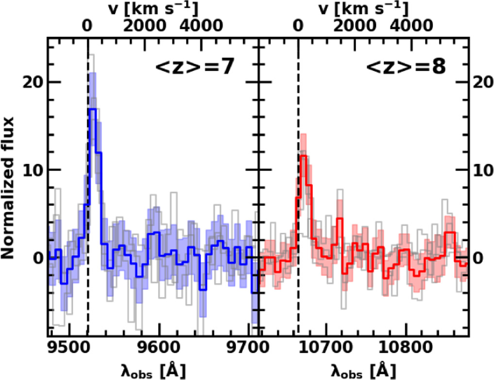
Figure 6. Lyα emission lines in the composite spectra of our sample galaxies. Left: the top and bottom axes present the velocity offset and observed wavelength. The y-axis corresponds to the fluxes normalized with the continuum fluxes. The blue solid line and shaded regions represent the composite spectrum for the 〈z〉 = 7 galaxies and associated 1σ errors, respectively. The gray solid lines show the individual spectra whose Lyα lines are redshifted to the mean redshift. The vertical black-dashed line denotes the Lyα wavelength in the observed frame defined with the mean redshift. Right: same as the left panel, but for the 〈z〉 = 8 galaxies. The red solid line indicates the composite spectrum for the 〈z〉 = 8 galaxies.
Download figure:
Standard image High-resolution image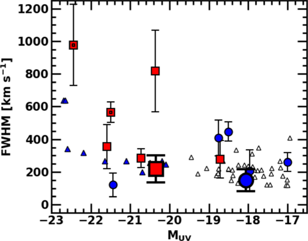
Figure 7. Lyα line width as a function of absolute UV magnitude. The large blue circles and large red squares represent the FHWMs measured from the composite spectra at 〈z〉 = 7 and 8, respectively. The small blue circles and small red squares denote the FHWMs of individual galaxies in our sample at z ∼ 7 and 8, respectively. The red double squares show the FWHMs of CEERS_01019 and GN-z11 (Bunker et al. 2023b) in our sample, both of which have signatures of AGN (Bunker et al. 2023b; Larson et al. 2023; Isobe et al. 2023b). The blue and white triangles indicate the FWHMs of the galaxies at z ∼ 7 (Ouchi et al. 2010; Endsley et al. 2022) and 2–3 (Hashimoto et al. 2017; Kerutt et al. 2022), respectively.
Download figure:
Standard image High-resolution image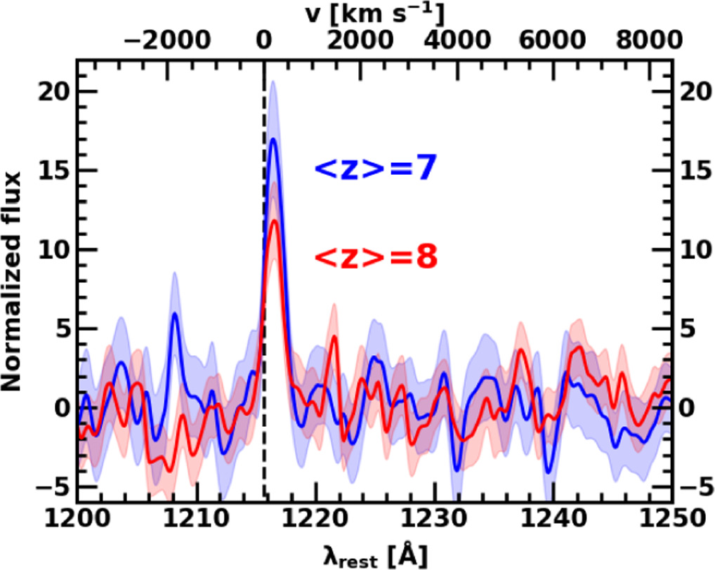
Figure 8. Evolution of Lyα line profiles. The top and bottom axes represent the velocity offset and rest-frame wavelength. The y-axis corresponds to the fluxes normalized with the continuum fluxes. The blue and red solid lines represent the composite spectra of the 〈z〉 = 7 and 8 galaxies, respectively. The light-shaded regions show the 1σ errors of the composite spectra. The vertical black-dashed line denotes the rest-frame Lyα wavelength.
Download figure:
Standard image High-resolution image3.4. Lyα EW
We obtain Lyα fluxes FLyα by the equation,
where  (
( ) is the maximum (minimum) value of the observed wavelength for the Lyα emission. We estimate flux errors from the MCMC results on the basis of the error spectrum made in Nakajima et al. (2023), Harikane et al. (2024), and Bunker et al. (2023a). The rest-frame Lyα EW, EW0,Lyα
is calculated with the equation,
) is the maximum (minimum) value of the observed wavelength for the Lyα emission. We estimate flux errors from the MCMC results on the basis of the error spectrum made in Nakajima et al. (2023), Harikane et al. (2024), and Bunker et al. (2023a). The rest-frame Lyα EW, EW0,Lyα
is calculated with the equation,
where fc
is the continuum fluxes at the observed wavelengths,  . For the galaxies with no FLyα
measurements (i.e., no Lyα detections), we estimate the upper limits of the Lyα fluxes. For each galaxy, we conduct Monte Carlo simulations with 100 mock spectra that are random realizations of the observed spectrum with the error spectrum. We conduct the model fitting to the 100 mock spectra to obtain Lyα flux measurements in the same manner as in Section 3.1, and determine the 1σ error of the Lyα flux with the distribution of the Lyα flux measurements of the 100 mock spectra. From these Lyα flux errors, we calculate the 3σ upper limits of EW0,Lyα
for the galaxies with no Lyα detections. We compare our measurements of EW0,Lyα
with those in the literature (Tang et al. 2023; Chen et al. 2024; Jones et al. 2024; Saxena et al. 2024) in Table 2 and find good agreement except for JADES_10013682, JADES_00004297, CEERS_80374, and CEERS_80239. For JADES_10013682, the EW0,Lyα
value measured in this study (31.5 ± 10.0 Å) is lower than those in Jones et al. (2024) (207 ± 27 Å) and Saxena et al. (2024) (337.2 ± 175.5 Å). While the EW0,Lyα
value of Jones et al. (2024) shown in Table 2 is derived by combining the Lyα flux measured from the grating spectrum in Saxena et al. (2024) and the continuum flux measured from the prism spectrum in Jones et al. (2024), our EW0,Lyα
value is derived based on the grating spectrum alone. Our measurement of the Lyα flux from the grating spectrum, (2.0 ± 0.2) × 10−18 erg s−1 cm−2, is consistent with that reported by Saxena et al. (2024), (2.2 ± 0.5) × 10−18 erg s−1 cm−2. For JADES_00004297, although the EW0,Lyα
value measured in this study (36.6 ± 5.0 Å) is lower than those in Jones et al. (2024) (122 ± 27 Å) and Saxena et al. (2024) (106.2 ± 22.5 Å), our measurement of the Lyα flux from the grating spectrum, (2.7 ± 0.4) × 10−18 erg s−1 cm−2, is consistent with that reported by Saxena et al. (2024), (2.7 ± 0.3) × 10−18 erg s−1 cm−2. We thus confirm that the differences in the EW0,Lyα
measurements of JADES_10013682 (JADES_00004297) come from the continuum fluxes obtained from the different resolutions of the grating and prism spectra, although our Lyα EW measurement is explained by the 2σ (3σ) error of those in Saxena et al. (2024). The impacts of the choice of the grating and prism spectra on Lyα EW measurements are discussed in Appendix A. For CEERS_80374, we do not detect Lyα emission at >3σ significance level and measure only 3σ upper limits of EW0,Lyα
, <86.7 Å, while Chen et al. (2024) report a Lyα detection with
. For the galaxies with no FLyα
measurements (i.e., no Lyα detections), we estimate the upper limits of the Lyα fluxes. For each galaxy, we conduct Monte Carlo simulations with 100 mock spectra that are random realizations of the observed spectrum with the error spectrum. We conduct the model fitting to the 100 mock spectra to obtain Lyα flux measurements in the same manner as in Section 3.1, and determine the 1σ error of the Lyα flux with the distribution of the Lyα flux measurements of the 100 mock spectra. From these Lyα flux errors, we calculate the 3σ upper limits of EW0,Lyα
for the galaxies with no Lyα detections. We compare our measurements of EW0,Lyα
with those in the literature (Tang et al. 2023; Chen et al. 2024; Jones et al. 2024; Saxena et al. 2024) in Table 2 and find good agreement except for JADES_10013682, JADES_00004297, CEERS_80374, and CEERS_80239. For JADES_10013682, the EW0,Lyα
value measured in this study (31.5 ± 10.0 Å) is lower than those in Jones et al. (2024) (207 ± 27 Å) and Saxena et al. (2024) (337.2 ± 175.5 Å). While the EW0,Lyα
value of Jones et al. (2024) shown in Table 2 is derived by combining the Lyα flux measured from the grating spectrum in Saxena et al. (2024) and the continuum flux measured from the prism spectrum in Jones et al. (2024), our EW0,Lyα
value is derived based on the grating spectrum alone. Our measurement of the Lyα flux from the grating spectrum, (2.0 ± 0.2) × 10−18 erg s−1 cm−2, is consistent with that reported by Saxena et al. (2024), (2.2 ± 0.5) × 10−18 erg s−1 cm−2. For JADES_00004297, although the EW0,Lyα
value measured in this study (36.6 ± 5.0 Å) is lower than those in Jones et al. (2024) (122 ± 27 Å) and Saxena et al. (2024) (106.2 ± 22.5 Å), our measurement of the Lyα flux from the grating spectrum, (2.7 ± 0.4) × 10−18 erg s−1 cm−2, is consistent with that reported by Saxena et al. (2024), (2.7 ± 0.3) × 10−18 erg s−1 cm−2. We thus confirm that the differences in the EW0,Lyα
measurements of JADES_10013682 (JADES_00004297) come from the continuum fluxes obtained from the different resolutions of the grating and prism spectra, although our Lyα EW measurement is explained by the 2σ (3σ) error of those in Saxena et al. (2024). The impacts of the choice of the grating and prism spectra on Lyα EW measurements are discussed in Appendix A. For CEERS_80374, we do not detect Lyα emission at >3σ significance level and measure only 3σ upper limits of EW0,Lyα
, <86.7 Å, while Chen et al. (2024) report a Lyα detection with  Å. For CEERS_80239, our measurements (105.3 ± 72.1 Å) are lower than those of Chen et al. (2024) (
 Å). These differences are due to the aperture used to extract the spectra. Our spectra are produced via the summation of 3 pixels (0
3) along the spatial direction centered on the spatial peak position to minimize the effects coming from the noisy regions close to the edge (Nakajima et al. 2023), while the spectra of Chen et al. (2024) are extracted with the aperture, which is typically 6 pixels. Because the apertures of our spectra are narrower than those of Chen et al. (2024), we may miss the extended fluxes of Lyα halos. Our measurements thus show no Lyα detection or a smaller EW0,Lyα
value than that of Chen et al. (2024). In Appendix B, we investigate the effects of the potential flux loss of the Lyα halo on our results. These different EW0,Lyα
measurements from those in the literature for a small number of galaxies may not affect our major results.
In Figure 9, we plot EW0,Lyα as a function of MUV. To investigate the redshift evolution of EW0,Lyα , we divide our sample into three subsamples by redshift so that each subsample has at least 10 galaxies and a redshift range of Δz ≳ 1. Our subsamples consist of 22, 12, and 17 galaxies whose redshift ranges are 6.5 ≤ z < 7.5, 7.5 ≤ z < 8.5, and 8.5 ≤ z < 13.5, referred to as z ∼ 7, 8, and 9–13, respectively. Note that we removed JADES_00008115 and CEERS_01163 from our subsamples because their MUV values are undetermined. We perform linear function fittings to our subsamples combined with samples of galaxies taken from the literature (Ono et al. 2012; Schenker et al. 2012; Oesch et al. 2015; Song et al. 2016; Shibuya et al. 2018; Matthee et al. 2019; Tilvi et al. 2020; Endsley et al. 2022; Jung et al. 2022; Kerutt et al. 2022; see Appendix C of Jones et al. 2024), which do not overlap with the galaxies in this study. For the 3σ upper limits of EW0,Lyα , we adopt two different distributions in the fittings. First, we adopt normal distributions with a mean value of 0 and standard deviations of the 1σ limits of EW0,Lyα . Second, we adopt uniform distributions between the 0 and 3σ upper limits of EW0,Lyα . We first fit the galaxies at z ∼ 7 to determine the slope and the intercept. We then use the fixed slope at z ∼ 7 and determine the intercept for the galaxies at z ∼ 8 and 9–13. The best-fit linear functions are presented in the top panel of Figure 9. There is no significant difference between the results using normal distributions and uniform distributions. We also conduct fittings based on the Kendall correlation test, using the cenken function in the NADA library from the R-project statistics package built based on the results of Akritas et al. (1995) and Helsel (2005). We use the cenken function because it computes the Kendall rank correlation coefficient and an associated linear function for censored data, such as a set of data, including upper limits. The fitting results using the cenken function are shown in the bottom panel of Figure 9. In both the top and bottom panels of Figure 9, we find that EW0,Lyα becomes lower at higher redshift, which is a clear signature of the redshift evolution of xH I with observational data alone. The evolution of Lyα EW is prominent between z ∼ 8 and 9–13, suggesting that reionization significantly proceeded between z ∼ 8 and 9–13. The p-values for the hypothesis that there is no correlation between MUV and EW0,Lyα at z ∼ 7, 8, and 9–13 are p = 0.58, 0.98, and 0.96, respectively. These p-values indicate that there is no clear correlation between MUV and EW0,Lyα at each redshift bin.
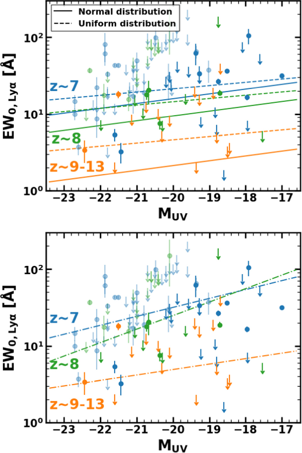
Figure 9. Rest-frame Lyα EW as a function of absolute UV magnitude. The blue, green, and orange circles (arrows) show the measurements (3σ upper limits) of the galaxies at z ∼ 7, 8, and 9–13 of our sample, respectively. The light blue, light green, and light orange symbols are the same as the blue, green, and orange symbols, but for the galaxies obtained from the literature (Ono et al. 2012; Schenker et al. 2012; Oesch et al. 2015; Song et al. 2016; Shibuya et al. 2018; Matthee et al. 2019; Tilvi et al. 2020; Endsley et al. 2022; Jung et al. 2022; Kerutt et al. 2022; see Appendix C of Jones et al. 2024). The top and bottom panels present the results of the linear and cenken function fittings, respectively. In the top panel, the solid (dashed) lines denote the best-fit linear functions obtained by adopting a normal (uniform) distribution for the EW0,Lyα upper limits. See Section 3.4 for the details of the fittings.
Download figure:
Standard image High-resolution image3.5. Lyα Fraction
To evaluate the ionizing state of the IGM, we calculate the Lyα fraction. We define the Lyα fraction  by the ratio of the number of galaxies with strong Lyα emission (EW > EWth) to the number of total galaxies. The Lyα fraction
  is typically investigated for galaxies with −21.75 < MUV < −20.25 and −20.25 < MUV < −18.75 (e.g., Stark et al. 2011; Ono et al. 2012; Schenker et al. 2012, 2014; Pentericci et al. 2018; Jones et al. 2024). We only have a small number of galaxies with −20.25 < MUV < −18.75 at z ∼ 8 and 9–13, and thus investigate the Lyα fraction at a rebinned redshift of z ∼ 7 and 8–13. For 12 (9) galaxies with −20.25 < MUV < −18.75 at z ∼ 7 (8–13), we find 3 (0) galaxies with EW > 25 Å. We obtain
  (3/12) and <0.19 (0/9) at z ∼ 7 and 8–13, respectively. We estimate the 1σ error and upper limit, using the statistics for small numbers of events by Gehrels (1986). As shown in the top panel of Figure 10, our
  value at z ∼ 7 is consistent with those in the literature (Ono et al. 2012; Schenker et al. 2012, 2014; Pentericci et al. 2018; Jones et al. 2024). We note that the denominators of
  (i.e., the LBGs) are confirmed via the photometry in the literature, while all of the galaxies used to calculate
  are spectroscopically confirmed in this work and Jones et al. (2024). Previous studies have indicated that
  increases with redshift at 4 ≤ z ≤ 6, while
  sharply decreases between z = 6 and 7. Our
  value is consistent with the trend of this sharp decrease in
  at 6 ≤ z ≤ 7, which is due to the poor Lyα transmission in the moderately neutral IGM. At z ∼ 8–13, we only obtain an upper limit of
  due to no galaxy with EW > 25 Å. Because the Lyα EW becomes lower at higher redshift, as shown in Figure 9, we need a lower threshold of EW than 25 Å to detect Lyα emitting galaxies at z ≳ 8. We thus calculate the Lyα fraction
  for galaxies with −20.25 < MUV < −18.75. We find one galaxy with EW > 10 Å at z ∼ 8−13 and obtain
  (3/12) and
  (1/9) at z ∼ 7 and 8–13, respectively. In the bottom panel of Figure 10, we find the trend of a decrease in the Lyα fraction at higher redshift between z ∼ 7 and 8–13. In summary, combining the results of
  in this work and the literature with those of
  in this work, we find that the Lyα fraction monotonically decreases from z ∼ 6 to 8–13 because of the more neutral hydrogen in the IGM at the earlier epoch of reionization. As for the xH I estimation, the full distribution (i.e., the probability distribution function) of Lyα EW allows us to place stronger constraints on xH I than on XLyα
(Treu et al. 2012, 2013; Mason et al. 2018), as described in Section 1. We thus mainly focus on xH I estimated with the probability distribution function (PDF) of Lyα EW in Section 4.
in this work, we find that the Lyα fraction monotonically decreases from z ∼ 6 to 8–13 because of the more neutral hydrogen in the IGM at the earlier epoch of reionization. As for the xH I estimation, the full distribution (i.e., the probability distribution function) of Lyα EW allows us to place stronger constraints on xH I than on XLyα
(Treu et al. 2012, 2013; Mason et al. 2018), as described in Section 1. We thus mainly focus on xH I estimated with the probability distribution function (PDF) of Lyα EW in Section 4.
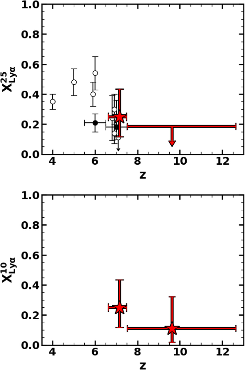
Figure 10. Lyα fraction as a function of redshift. Top: the red star mark and black circles indicate the  values obtained from the galaxies, all of which are spectroscopically confirmed in this work and Jones et al. (2024), respectively. The red arrow denotes the same as the red star mark, but for the upper limit of
  . The white circles represent the
  values obtained from the galaxies, including those confirmed via the photometry in the literature (Stark et al. 2011; Ono et al. 2012; Schenker et al. 2012, 2014; Pentericci et al. 2018; Mason et al. 2019). Bottom: the red star marks show the
  values obtained in this work.
Download figure:
Standard image High-resolution image4. Estimates of the Neutral Hydrogen Fraction
We estimate neutral hydrogen fractions xH I, comparing the rest-frame Lyα EW values (simply referred to as EW in this section) obtained from observations with those of the theoretical EW distribution models developed by Dijkstra et al. (2011). As shown in Figure 11, EW values at the low xH I universe are higher than those at the high xH I universe, due to the Lyα damping wing absorption made by the IGM. In the EW distribution models, Dijkstra et al. (2011) quantify the PDF of the fraction of Lyα photons transmitted through the IGM TIGM, combining galactic outflow models with large-scale seminumeric simulations of reionization. There are two parameters, the neutral hydrogen column density NH I and the outflow velocity vwind, in the galactic outflow models. The EW distribution models are constructed under the assumption that the IGM at z = 6 is completely transparent to Lyα photons, and that the PDF of EW changes only by the evolution of the ionization state of the IGM. It is also assumed that the EW distribution at z = 6 is described by an exponential function,  , where EWc is a scale factor of EW at z = 6. The EW distributions during the epoch of reionization are computed with
  where N is a normalization factor, and p(TIGM) is a PDF of TIGM, which is computed in Dijkstra et al. (2011). As a fiducial model, Dijkstra et al. (2011) use a set of the models with NH I = 1020 cm−2, vwind = 200 km s−1, and EWc = 50 Å, in which TIGM is computed at z ∼ 8.6. For comparison, we show the models of EW distribution with NH I = 1020 cm−2, vwind = 25 and 200 km s−1, and EWc = 30, 40, and 50 Å in Figure 11. The EW distribution does not largely change for different vwind values, but moderately changes for different EWc values. Because Dijkstra et al. (2011) find the relation of ΔvLyα
∼ 2vwind in the galactic outflow model, the Lyα velocity offset of the models with vwind = 200 km s−1 corresponds to 400 km s−1. We note that the lower Lyα velocity offsets in our sample of ΔvLyα
= 234 ± 76 km s−1 (mean values; Section 3.2) than that of the models are unlikely to affect our estimates because vwind does not largely change the EW distribution, as shown in the top panel of Figure 11. Recent observational studies show column densities of neutral gas of high-z galaxies (Heintz et al. 2023; Umeda et al. 2023), which are NH I ∼ 1019–1023 cm−2. The observed values of NH I are comparable to those of the models. Dijkstra et al. (2011) chose a scale factor of EWc = 50 Å because the Lyα fraction of LAEs with EW > 75 Å estimated with the EWc value is about 0.2, which corresponds to the median value observed at z ∼ 6 (Stark et al. 2010). However, Pentericci et al. (2018) claim that a scale factor of a best-fit exponential function that matches the observations at z ∼ 6 is EWc = 32 ± 8 Å. Mason et al. (2018) parameterize the z ∼ 6 EW distribution (De Barros et al. 2017; Pentericci et al. 2018) as an exponential function plus a delta function, which depend on UV magnitude and obtain the scale factor of
where N is a normalization factor, and p(TIGM) is a PDF of TIGM, which is computed in Dijkstra et al. (2011). As a fiducial model, Dijkstra et al. (2011) use a set of the models with NH I = 1020 cm−2, vwind = 200 km s−1, and EWc = 50 Å, in which TIGM is computed at z ∼ 8.6. For comparison, we show the models of EW distribution with NH I = 1020 cm−2, vwind = 25 and 200 km s−1, and EWc = 30, 40, and 50 Å in Figure 11. The EW distribution does not largely change for different vwind values, but moderately changes for different EWc values. Because Dijkstra et al. (2011) find the relation of ΔvLyα
∼ 2vwind in the galactic outflow model, the Lyα velocity offset of the models with vwind = 200 km s−1 corresponds to 400 km s−1. We note that the lower Lyα velocity offsets in our sample of ΔvLyα
= 234 ± 76 km s−1 (mean values; Section 3.2) than that of the models are unlikely to affect our estimates because vwind does not largely change the EW distribution, as shown in the top panel of Figure 11. Recent observational studies show column densities of neutral gas of high-z galaxies (Heintz et al. 2023; Umeda et al. 2023), which are NH I ∼ 1019–1023 cm−2. The observed values of NH I are comparable to those of the models. Dijkstra et al. (2011) chose a scale factor of EWc = 50 Å because the Lyα fraction of LAEs with EW > 75 Å estimated with the EWc value is about 0.2, which corresponds to the median value observed at z ∼ 6 (Stark et al. 2010). However, Pentericci et al. (2018) claim that a scale factor of a best-fit exponential function that matches the observations at z ∼ 6 is EWc = 32 ± 8 Å. Mason et al. (2018) parameterize the z ∼ 6 EW distribution (De Barros et al. 2017; Pentericci et al. 2018) as an exponential function plus a delta function, which depend on UV magnitude and obtain the scale factor of ![${\mathrm{EW}}_{{\rm{c}}}=31+12\tanh [4({M}_{\mathrm{UV}}+20.25)]$](https://content.cld.iop.org/journals/0004-637X/967/1/28/revision1/apjad38c2ieqn126.gif) Å, which corresponds to about 30 Å for the MUV values of our sample. We thus use the sets of models with NH I = 1020 cm−2, vwind = 200 km s−1, and EWc = 35 ± 5 Å, which are comparable to the observed values.
Å, which corresponds to about 30 Å for the MUV values of our sample. We thus use the sets of models with NH I = 1020 cm−2, vwind = 200 km s−1, and EWc = 35 ± 5 Å, which are comparable to the observed values.
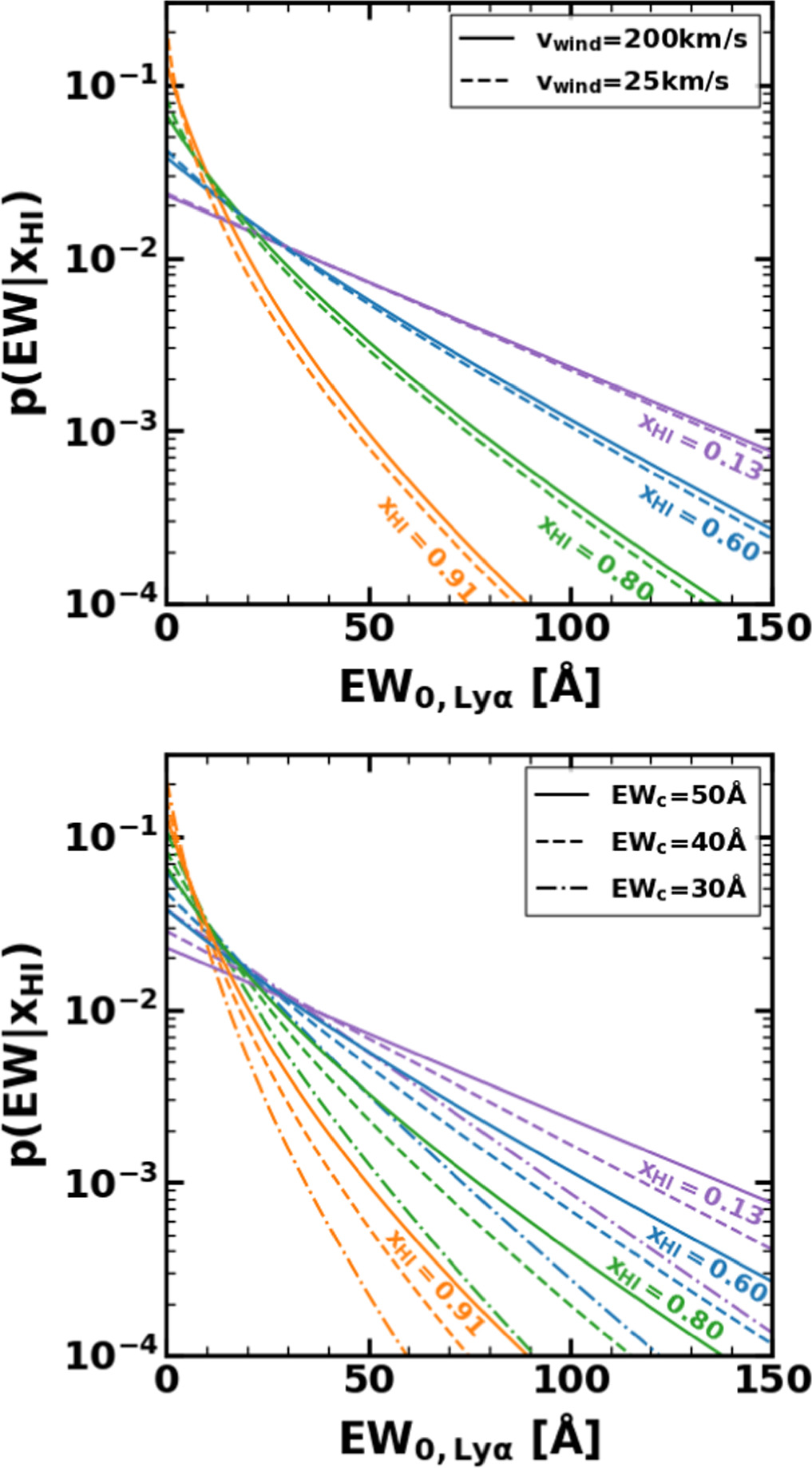
Figure 11. Probability distribution functions of the rest-frame Lyα EW. The purple, blue, green, and orange solid lines indicate the EW distribution models (Dijkstra et al. 2011) with a neutral hydrogen column density NH I = 1020 cm−2, an outflow velocity vwind = 200 km s−1, a scale factor EWc = 50 Å, and neutral hydrogen fractions xH I = 0.13, 0.60, 0.80, and 0.91, respectively. In the top panel, the dashed lines represent the same as the solid lines, but for the models with vwind = 25 km s−1. In the bottom panel, dashed (dashed–dotted) lines denote the same as the solid lines, but for the models with EWc = 40 (30) Å.
Download figure:
Standard image High-resolution imageFigure 12 presents the MUV distribution as a function of redshift for our sample. We find that there is a trend that faint galaxies are included for our galaxies in the low-redshift bins. To avoid systematics introduced by bias in UV magnitudes, we select galaxies, removing 8 (1) galaxies at z ∼ 7 (8) fainter than characteristic luminosity with the criterion of z < 7 or MUV > −18. We conduct two sample Kolmogorov–Smirnov tests between the UV magnitudes for the galaxies of our subsamples (Section 3.4) before and after the selection. Note that the redshift range of our subsamples for z ∼ 7 after the selection is 7 ≤ z < 7.5. We confirm that the UV magnitude distributions are not similar between the galaxies at z ∼ 7 and ∼ 8 before the selection at the 99% significance level, but consistent for all three redshift bins after the selection at the 99% significance level. We estimate xH I for our subsamples of z ∼ 7, 8, and 9–13, which consist of 14 (=22 −8), 11 (=12 −1), and 17 galaxies, respectively (Section 3.4).
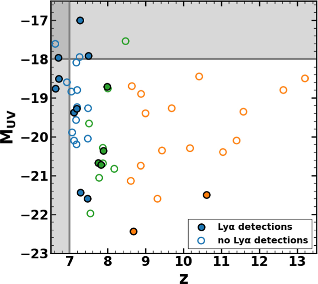
Figure 12. Absolute UV magnitude distribution of our sample galaxies as a function of redshift. The blue, green, and orange-filled (open) circles denote galaxies with (no) Lyα detections at z ∼ 7, 8, and 9–13, respectively. The gray solid lines represent the selection criteria for our sample (Section 4).
Download figure:
Standard image High-resolution imageHere, we need to be careful about the effects of the slit loss on the Lyα EW measurements because we compare the Lyα EW obtained from JWST/NIRSpec MSA observations with the theoretical models of Lyα EW distributions based on the Very Large Telescope/FORS2 observations (Pentericci et al. 2018) to estimate xH I. Our sample galaxies are observed with an NIRSpec MSA microshutter, which could miss the fluxes of extended Lyα halos due to the small area of the microshutters (020 × 0
46) (Jakobsen et al. 2022) compared to the FORS2 slit (∼1″ × 8″) (Pentericci et al. 2018). The slit loss effects on Lyα emission are discussed in recent studies. While Jung et al. (2023) claim that the Lyα flux of one source measured from NIRSpec MSA is only 20% of those measured from MOSFIRE, Tang et al. (2023) find that the Lyα EWs of four sources measured from NIRSpec MSA are consistent with those measured from ground-based observations. Jones et al. (2024) also show that the Lyα EW measurements from NIRSpec MSA are not likely to affect their results. In addition, our
 value obtained from NIRSpec MSA observations is consistent with that obtained from FORS2 observations (Pentericci et al. 2018), suggesting that slit loss effects on Lyα EW measurements may not be significant. However, we need to quantitatively assess the slit loss effects on Lyα EW measurements to estimate xH I accurately. As done by Tang et al. (2024), we conducted a forward-modeling analysis to compare the Lyα EW obtained from NIRSpec MSA with those from FORS2. The details of the analysis are described in Appendix B. The results show that Lyα EW measured with NIRSpec MSA is 72% ± 8% of those with FORS2. We thus use the corrected Lyα EWs divided by this fraction (72% ± 8%) as fiducial values to estimate xH I.
To estimate the probability distributions of xH I, we perform a Bayesian inference based on that of Mason et al. (2018). We note that our Bayesian method only sets xH I as a free parameter, instead of xH I and MUV in the method of Mason et al. (2018) because our subsamples at each redshift bin have similar distributions of UV magnitude as described above. Under the Bayesian method, the posterior probability distribution p(xH I∣EW) is based on the equation,

where EWi represents EW measurements of individual galaxies. Here, p(EWi ∣xH I) is a likelihood function, and p(xH I) is a uniform prior with 0 ≤ xH I ≤ 1. The likelihood functions are calculated, including the measured 1σ errors σi by the equation,
where p(EW∣xH I) represents the EW distribution model as a function of xH I. For galaxies with no Lyα detections, we instead use the likelihood functions, including the 3σ upper limits of EWlim given by
where erfc(x) is the complementary error function for x.
Combining Equations (4)–(6), we calculate the posterior distributions of xH I. As described above, we use the EW distribution models with NH I = 1020 cm−2, vwind = 200 km s−1, and EWc = 35 ± 5 Å. The uncertainties for the scale factor of EWc = 35 ± 5 Å in the EW distribution models are taken into account according to the following steps. First, we calculate the posterior distributions for each of the EWc values in the ΔEWc = 1 Å bins. We then take averages of the posterior distributions, using normal distributions with EWc = 35 ± 5 Å. The posterior distributions of xH I at each redshift bin are shown in Figure 13. We determine the xH I values and 1σ errors from the posterior distributions in the same manner as in Section 3.1. The xH I values estimated with the corrected EWs are xH I < 0.79,  , and
, and  at z ∼ 7, 8, and 9–13, respectively. We present a 3σ upper limit for xH I at z ∼ 7. For comparison, we also estimate xH I with two sets of models and measurements. One is the combination of the EW distribution models of Dijkstra et al. (2011) and the uncorrected EWs. The other is the combination of the EW distribution models of Mason et al. (2018, see their Figure 7) with the corrected EWs. As described above, the z ∼ 6 EW distribution in Mason et al. (2018) is based on an LAE observation with FORS2 (De Barros et al. 2017; Pentericci et al. 2018). We thus estimate xH I by combining the corrected EWs with the models of Mason et al. (2018). In Figure 14, we present the results with the three different sets of models and EWs. The xH I estimates with uncorrected EWs are modestly overestimated compared to those with corrected EWs. In the case where we use corrected EWs, there are little differences between the xH I estimates with EW distribution models of Dijkstra et al. (2011) and those of Mason et al. (2018). We thus adopt the xH I estimates with the EW distribution models of Dijkstra et al. (2011) and corrected EWs as fiducial results.
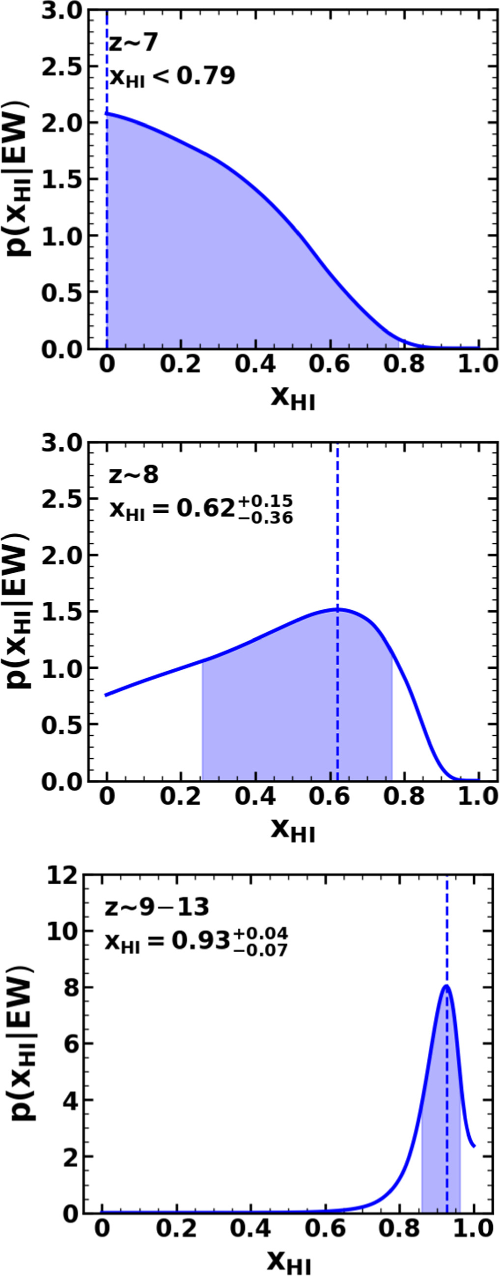
Figure 13. Posterior distributions of xH I at z ∼ 7 (top), 8 (middle), and 9–13 (bottom). The dashed lines show the mode, while the shaded regions represent the 99.7th, 68th, and 68th percentile HPDI at z ∼ 7, 8, and 9–13, respectively. The estimated values are xH I < 0.79,  , and
, and  at z ∼ 7, 8, and 9–13, respectively.
Download figure:
Standard image High-resolution image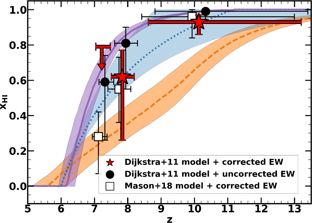
Figure 14. Comparison of the redshift evolution of xH I. The red star marks, black circles, and white squares represent xH I estimates obtained with the Dijkstra et al. (2011) models+corrected Lyα EW, the Dijkstra et al. (2011) models+uncorrected Lyα EW, and the Mason et al. (2018) models+corrected Lyα EW, respectively. The purple solid, blue-dotted, and orange-dashed lines represent the reionization scenarios suggested by Naidu et al. (2020), Ishigaki et al. (2018), and Finkelstein et al. (2019), respectively. The light-shaded regions show the uncertainties of the reionization scenarios.
Download figure:
Standard image High-resolution image5. Discussion
In Figure 15, we present our constraints on the redshift evolution of xH I at z = 7–13. For comparison, we also show the xH I estimates taken from the literature. Our xH I values are consistent with those estimated with Lyα damping wing absorption of QSOs/gamma-ray bursts (GRBs), Lyα luminosity function, Lyα EW of LBGs, and the Thomson scattering optical depth of the CMB within the errors. While these results constrain xH I up to z ∼ 7.5, which is limited to the redshifts of the identified QSOs and GRBs (Totani et al. 2014; Wang et al. 2019; Matsuoka et al. 2023), a recent study by Umeda et al. (2023) extends the xH I measurements to z ∼ 8–12 with JWST galaxies via UV continuum modeling of the Lyα damping wing absorption features. The sample of Umeda et al. (2023) consists of 26 galaxies, which are used in their Lyα damping wing analysis, while our sample of 53 galaxies includes all 26 of Umeda et al.'s galaxies. Although there is an overlap of the samples between our study and Umeda et al.'s study, our study focuses on Lyα line EW statistics compared with the numerical simulations, which complement the study of Umeda et al. (2023) in the independent method to estimate xH I. We confirm that the xH I estimates of our study and Umega et al.'s study are consistent within the errors. This consistency solidifies the validity of our measurements of Lyα EW, which is used to infer the xH I values. We plot the late, medium-late, and early scenarios suggested by Naidu et al. (2020), Ishigaki et al. (2018), and Finkelstein et al. (2019), respectively (Section 1). Our results are consistent with the late and medium-late scenarios.
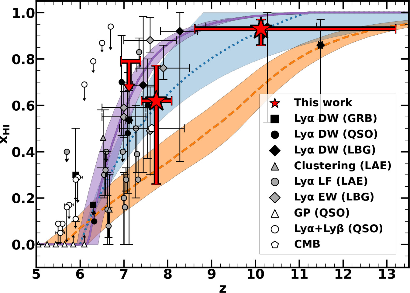
Figure 15. Redshift evolution of xH I. The red star marks denote fiducial xH I estimates obtained in this work. The purple solid, blue-dotted, and orange-dashed lines represent the reionization scenarios suggested by Naidu et al. (2020), Ishigaki et al. (2018), and Finkelstein et al. (2019), respectively. The light-shaded regions show the uncertainties of the reionization scenarios. The black squares, circles, and diamonds present the xH I estimates derived from Lyα damping wing absorption of GRBs (Totani et al. 2006, 2014), QSOs (Schroeder et al. 2013; Davies et al. 2018; Greig et al. 2019; Wang et al. 2020), and LBGs (Curtis-Lake et al. 2023; Hsiao et al. 2023; Umeda et al. 2023), respectively. The gray triangles and circles indicate the xH I estimates using an LAE clustering analysis (Ouchi et al. 2018; Umeda 2023) and Lyα luminosity function (Ouchi et al. 2010; Konno et al. 2014; Inoue et al. 2018; Morales et al. 2021; Goto et al. 2021; Ning et al. 2022; Umeda 2023), respectively. The gray diamonds denote the xH I estimates obtained from the Lyα EW distribution of LBGs (Hoag et al. 2019; Mason et al. 2019; Jung et al. 2020; Whitler et al. 2020; Bruton et al. 2023; Morishita et al. 2023). The white triangles and circles represent the xH I estimates derived from the Gunn–Peterson through of QSOs (Fan et al. 2006) and Lyα and Lyβ forest dark fractions of QSOs (McGreer et al. 2015; Zhu et al. 2022; Jin et al. 2023), respectively. The white pentagon shows the xH I estimates obtained from the CMB observations under the assumption of instantaneous reionization (Planck Collaboration et al. 2020).
Download figure:
Standard image High-resolution imageAs explained in Section 1, the late and medium-late scenarios suggest that sources of reionization form at the late epoch, probably at z ∼ 7–8. If the late scenario is correct, the slopes of UV luminosity functions should be as shallow as α > −2 under the assumption that fesc depends on the SFR surface density ΣSFR (Section 1). However, recent observational results have preferred a steep slope of α < −2 (Bouwens et al. 2017; Livermore et al. 2017; Atek et al. 2018; Ishigaki et al. 2018; Finkelstein et al. 2019). Because the requirement of the shallow UV slope does not agree with the observational results, this discrepancy could possibly suggest that the escape fraction does not depend on ΣSFR but on the other quantities. For example, if the escape fraction positively correlates with halo masses (e.g., Gnedin et al. 2008; Wise & Cen 2009; Sharma et al. 2016), the positive correlation could lead to late reionization with the steep UV slope suggested by the UV luminosity function observations. If we consider the possibility of star-forming galaxies as major sources of reionization, ionizing photons are prevented from escaping to the IGM because of the enrichment of metals and dust in star-forming galaxies. To account for the high escape fractions of star-forming galaxies hosted by moderately massive halos, channels in the ISM produced by the starbursts and frequent supernovae (e.g., Paardekooper et al. 2015; Steidel et al. 2018) or unknown physical processes may be needed. In fact, Paardekooper et al. (2015) show that young star-forming galaxies in massive halos would have a high escape fraction if supernova feedback causes either an inhomogeneous density or the removal of the dense gas around the galaxies. Another possibility may be that galaxies in massive halos harbor AGNs that efficiently produce ionizing photons. While QSOs (i.e., bright AGNs) make negligible contributions to reionization due to their low number density (Onoue et al. 2017; McGreer et al. 2018; Parsa et al. 2018; Wang et al. 2019; Jiang et al. 2022), some studies suggest that the contributions from faint AGNs to reionization may be significant (Giallongo et al. 2015; Haardt & Salvaterra 2015; Giallongo et al. 2019). In fact, many faint AGNs have been found at z = 4–10 by JWST observations (Harikane et al. 2023; Kocevski et al. 2023; Maiolino et al. 2023a, 2024; Übler et al. 2023; Matthee et al. 2024). Harikane et al. (2023) and Maiolino et al. (2023a) suggest that the contributions from faint AGNs (MUV ≳ −22) to the ionizing photons are not very large but do exist. Such many faint AGNs may have caused the late reionization. In summary, our results, together with recent observational results, suggest that the escape fraction may positively correlate with halo masses and that possible major sources of reionization are star-forming galaxies or faint AGNs hosted by moderately massive halos. In fact, the galaxies with high neutral hydrogen column densities, which disturb the escape of ionizing photons, are found at z ≳ 8 (D’Eugenio et al. 2023; Heintz et al. 2023; Umeda et al. 2023), indicating that significant reionization is caused by the objects that emerge at the late era of reionization (z ∼ 7–8) and are hosted by moderately massive halos.
6. Summary
In this paper, we present our constraints on xH I from Lyα EWs of galaxies at z ∼ 7–13. We select 54 galaxies at 6.6 < z < 13.2 observed with JWST/NIRSpec in the multiple programs of ERS, DDT, GO, and GTO. The redshifts of the galaxies of our sample are spectroscopically confirmed by emission lines or spectral breaks. Because we are not able to conduct spectral fitting for one galaxy, we investigate the Lyα properties of 53 galaxies. We obtain the Lyα velocity offset, line width, and EW for 15 galaxies with Lyα detections from the spectral fittings. For 38 galaxies with no Lyα detections, we measure the 3σ upper limits of Lyα EW. Our major findings are summarized below:
- 1.We find no redshift evolution of the Lyα velocity offset and line width from z ∼ 2–3 to ∼ 7–13. While the composite spectra at mean redshifts of 〈z〉 = 7 and 8 also show no evolution of line profiles, we find a clear attenuation of line flux, suggesting the evolution of the Lyα EW. To investigate the redshift dependence of the Lyα EW, we conduct linear function fittings for galaxies at z ∼ 7, 8, and 9–13 by adopting various probability distributions for the upper limits of Lyα EW. We find that EW0,Lyα becomes lower at higher redshift (Figure 9), which is a clear signature of the redshift evolution of xH I based on the observational data alone. The Lyα fraction measurements at z ∼ 7 also suggest the evolution of xH I between z ∼ 6 and 7.
- 2.To estimate xH I independent of UV magnitude, we select 42 out of 53 galaxies with z ≥ 7 and MUV ≤ −18 that have similar distributions of MUV for each redshift bin. We estimate xH I by comparing our EW0,Lyα values with those of the EW distribution models (Dijkstra et al. 2011) based on a Bayesian inference (Mason et al. 2018). We correct our EW0,Lyα values by forward modeling the slit loss effects for comparison with ground-based results. The estimates are xH I < 0.79,
 , and at z ∼ 7, 8, and 9–13, respectively. Our xH I values are consistent with those estimated with the Lyα damping wing absorption of QSOs/GRBs, Lyα luminosity function, Lyα EW of LBGs, and the Thomson scattering optical depth of the CMB within errors. Our xH I values are also consistent with those estimated in a complementary approach with the UV continua of bright galaxies for damping absorption estimates (Umeda et al. 2023). The redshift evolution of our xH I values is consistent with the late or medium-late reionization scenarios. Such a late reionization history suggests that major reionization sources are the objects hosted by moderately massive halos, which is in contrast to the widely accepted picture of abundant faint low-mass objects for reionization sources.


Acknowledgments
We thank the anonymous referee for the valuable comments that greatly improved this manuscript. We thank Mark Dijkstra for providing us with the machine-readable table of their simulation results. We thank Roland Bacon, Pratika Dayal, Yoshinobu Fudamoto, Takuya Hashimoto, Kohei Inayoshi, Akio Inoue, Daichi Kashino, Satoshi Kikuta, Takanobu Kirihara, Haruka Kusakabe, Pascal Oesch, Kazuyuki Omukai, Laura Pentericci, and Hidenobu Yajima for the valuable discussions on this work. This work is based on observations made with the NASA/ESA/CSA JWST. The data were obtained from the Mikulski Archive for Space Telescopes at the Space Telescope Science Institute, which is operated by the Association of Universities for Research in Astronomy, Inc., under NASA contract NAS 5-03127 for JWST. The specific observations analyzed can be accessed via the MAST website (doi:10.17909/8tdj-8n28). These observations are associated with programs ERS-1324 (GLASS), ERS-1345 (CEERS), GO-1433, DDT-2750, and GTO-1210 (JADES). The authors acknowledge the GLASS, CEERS, GO-1433, and DDT-2750 teams led by Tommaso Treu, Steven L. Finkelstein, Dan Coe, and Pablo Arrabal Haro, respectively, for developing their observing programs with a zero-exclusive-access period. We thank the JADES team for publicly releasing reduced spectra and catalogs from the JADES survey. This publication is based upon work supported by the World Premier International Research Center Initiative (WPI Initiative), MEXT, Japan, and KAKENHI (20H00180, 21H04467) through the Japan Society for the Promotion of Science. This work was supported by the joint research program of the Institute for Cosmic Ray Research (ICRR), University of Tokyo.
Software: NumPy (Harris et al. 2020), matplotlib (Hunter 2007), SciPy (Virtanen et al. 2020), Astropy (Astropy Collaboration et al. 2013, 2018, 2022), and emcee (Foreman-Mackey et al. 2013).
Appendix A: Comparison of Lyα EW Measured with the Grating and Prism Spectra
In this study, we measure Lyα EW with the grating and prism spectra. Recent studies of LAEs observed with JWST show that Lyα emission is not detected with prism spectra, but detected with grating spectra (e.g., Bunker et al. 2023b; Saxena et al. 2024). However, Lyα EWs obtained from our grating spectra are consistent with Lyα EWs or the 3σ upper limits of the Lyα EW obtained from our prism spectra except for one source, JADES_10013682, as shown in Figure A1. Although the Lyα EW measurements of JADES_10013682 with the prism spectra are higher than those with the grating spectra, which is explained by 2σ errors. Including Lyα EW measurements with the prism spectra in our analysis thus would not affect our results significantly.
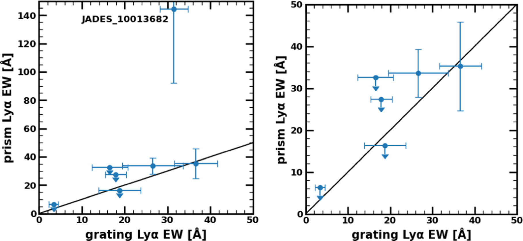
Figure A1. Comparison of Lyα EW measurements with our grating spectra and those with our prism spectra. The left panel presents a wide range of the figure, while the right panel zooms in to show the plots more clearly. The circles denote Lyα EWs for sources observed with both the grating and prism. The error bars and arrows represent the 1σ errors and 3σ upper limits, respectively. The black line indicates that Lyα EWs obtained from grating spectra are equivalent to those obtained from prism spectra.
Download figure:
Standard image High-resolution imageAppendix B: Forward Modeling
As described in Section 4, we conduct a forward-modeling analysis to estimate the slit loss effects on Lyα EW measurements. We first obtain the intrinsic UV and Lyα spatial profile of 10 galaxies at z ∼ 5–6 based on measurements with MUSE (Leclercq et al. 2017). For UV continuum emission, we construct a 2D exponential profile with a scale length of a core rscont and a total UV flux obtained from the UV magnitude. For Lyα emission, we construct a 2D exponential profile for two components, which are a core component and a halo component. The profile of the core (halo) component is obtained from a scale length of the core rscont (halo rshalo) and a total core (halo) Lyα flux Fcont (Fhalo). We then convolve the UV and Lyα profiles with the point-spread function (PSF) of NIRSpec and FORS2. We assume that the PSF is approximated by a 2D Gaussian profile. The PSF of NIRSpec is obtained from the WebbPSF package (Perrin et al. 2014). We adopt a seeing size of ∼08 (Pentericci et al. 2018) as the FWHM of the PSF of FORS2. In Figure B1, we present an example of the forward modeling for a source at z ∼ 5. For NIRSpec, we measure Lyα and UV fluxes by summing the fluxes within the aperture size of 0
3 (Section 3.4) along the spatial direction centered on the spatial peak position of the slit (0
20 × 0
46; Jakobsen et al. 2022). For FORS2, we measure the fluxes by summing the fluxes within the slit (1″ × 8″; Pentericci et al. 2018). We vary the offset of the source from the center of the slit along the diagonal line of the NIRSpec MSA slit for both the NIRSpec MSA and FORS2 slits. From the flux measurements with NIRSpec and FORS2, we obtain the Lyα EW of 10 galaxies at z ∼ 5–6. We calculate 1σ Lyα EW errors by conducting Monte Carlo simulations of 100 forward modelings with the errors of rscont, rshalo, Fcont, and Fhalo. We present the fractions of Lyα EW measured within the NIRSpec MSA (FORS2) slit to the Lyα EW measured with the total Lyα and UV fluxes, and fractions of Lyα EW measurements with NIRSpec to those with FORS2 for different source positions in the left and right panels of Figure B2, respectively. We confirm that the fractions do not depend on the source's position in the slit. We thus adopt the fraction of Lyα EW measurements with NIRSpec to those with FORS2 where the source is in the center of the slit, 72% ± 8%, as a correction factor in Section 4.
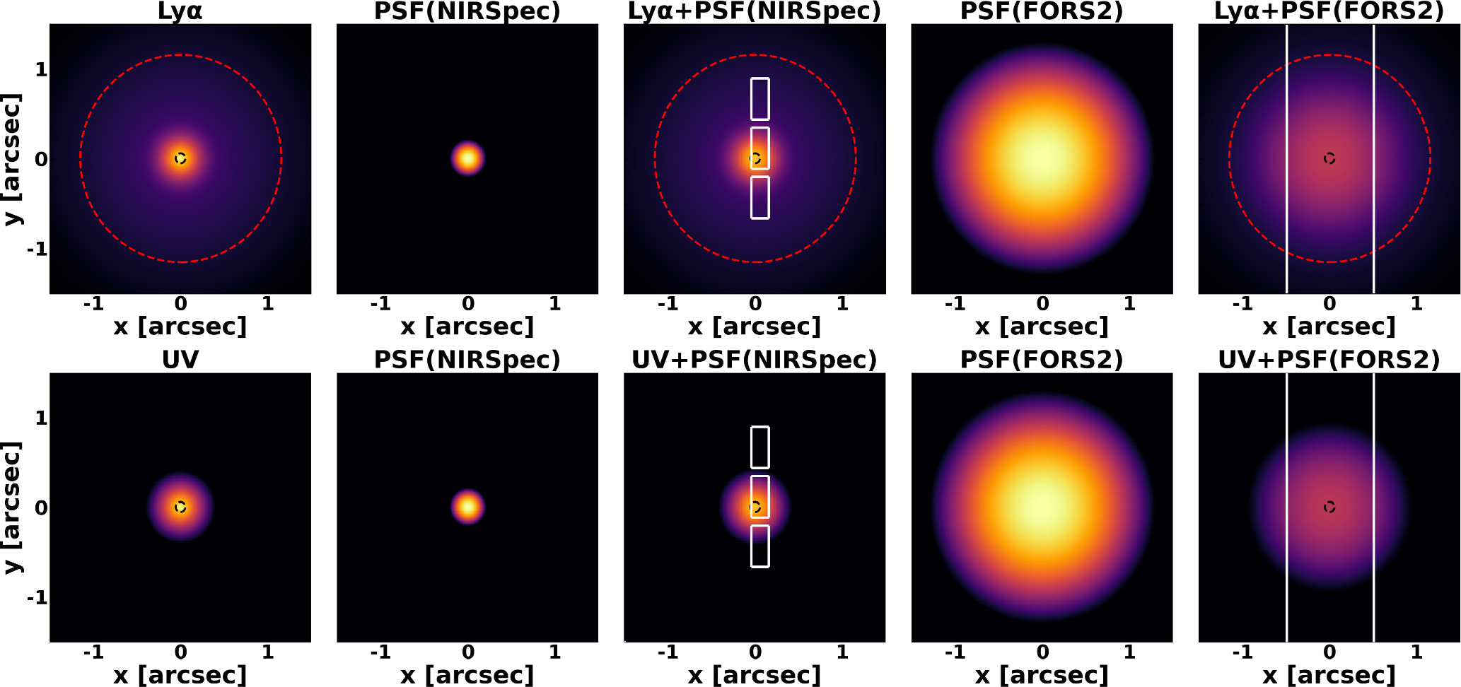
Figure B1. Example of the forward modeling of a source at z ∼ 5. From left to right in the top row, each panel indicates the intrinsic Lyα spatial profile, PSF of NIRSpec, Lyα emission convolved with the PSF of NIRSpec, PSF of FORS2, and Lyα emission convolved with the PSF of FORS2. The bottom row shows the same as the top row but for UV emission. The radius of the black-dashed and red-dashed circles correspond to the scale lengths of the core and halo components, respectively. The white lines represent the NIRSpec MSA three-shutter slits (middle panel) and FORS2 slits (rightmost panel).
Download figure:
Standard image High-resolution image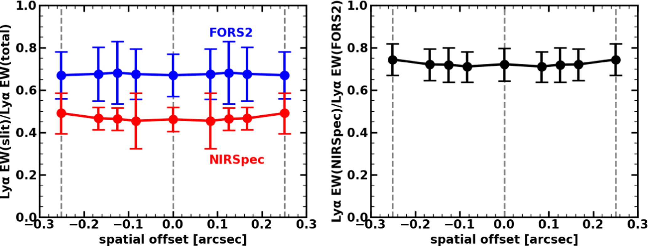
Figure B2. The fraction of Lyα EW as a function of the source position. Left: the red (blue) circles represent the fractions of Lyα EW measured within the NIRSpec MSA (FORS2) slit to Lyα EW measured with total Lyα and UV fluxes. The left, middle, and right gray-dashed lines indicate the corner, center, and corner of the slit, respectively. Right: the black circles denote the fractions of Lyα EW measurements with NIRSpec to those with FORS2. The gray-dashed lines show the same as the top panel.
Download figure:
Standard image High-resolution image